Real-Time Implementation of a LQR-Based Controller for the Stabilization of a Double Inverted Pendulum

(1)

Real-Time Implementation of a LQR-Based

Controller for the Stabilization of a Double

Inverted Pendulum

Amanda Bernstein and Hien Tran,

Member, SIAM

Abstract—The problem of real-time implementation of a linear quadratic regulator (LQR)-based controller for the balance of a double inverted pendulum (DIP) mounted on a cart is presented. Physically, the DIP system is stabilized when the two pendulums are aligned in a vertical position. The mathematical model for the dynamics of a DIP can be derived using the Lagrange’s energy method, which is computed from the calculation of the total potential and kinetic energies of the system. This results in a highly nonlinear system of three second-order ordinary differential equations. The nonlinear system is linearized around its zero equilibrium state and LQR controller is implemented in real-time to stabilize the DIP system (i.e., to keep DIP in an upright position). Both simulation and real-time experimental results are presented.

Index Terms—double inverted pendulum, LQR, feed-back controller, real-time implementation.

I. INTRODUCTION

T

HE double inverted pendulum (DIP) system is an extension of the single inverted pendulum (with one additional pendulum added to the single inverted pendulum), mounted on a moving cart. The DIP sys-tem is a standard model of multivariable, nonlinear, unstable system, which can be used for pedagogy as well as for the introduction of intermediate and advanced control concepts. There are two types of control synthesis for an inverted pendulum, swing-up and stabilization. One of the most popular control methods for swinging up the inverted pendulum is based on the energy method (see [1] and the refer-ences therein). The stabilization problem of an inverted pendulum is a classical control example for testing of linear and nonlinear controllers (see, e.g., [1], [2], [3]). Several control design approaches have been applied for the stabilization of the double inverted pendulum including the linear quadratic regulator [4], the state-dependent Riccati equation, optimal neural network [5], and model predictive control [3]. To our knowl-edge, these studies only use numerical simulations to

Manuscript received December 12, 2016.

A. Bernstein is a graduate student with the Department of Mathematics, North Carolina State University, Raleigh, NC 27695 USA e-mail: [email protected].

[image:1.595.357.471.214.366.2]

H. Tran is with the Department of Mathematics, North Carolina State University, Raleigh, NC 27695 USA e-mail: [email protected].

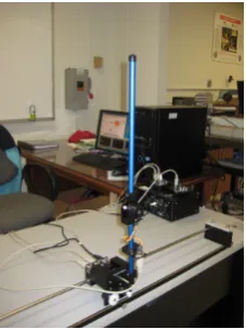
Fig. 1: Double inverted pendulum mounted on a Quanser linear servo base unit (IP02).

test the feasibility of the control methodologies and do not provide real-time experimental implementation on a physical system.

In this paper, we present the real-time implementa-tion of a LQR-based feedback control for the stabiliza-tion about the upright posistabiliza-tion of the double inverted pendulum mounted on a cart. The apparatus of the DIP system, which was provided by Quanser Consulting Inc. (119 Spy Court, Markham, Ontariio, L3R 5H6, Canada), is depicted in Fig. 1. The DIP system consists of two aluminum rods; one seven inches long and the other 12 inches long. The aluminums are mounted on the linear servo base unit (IP02) consisting of a cart driven by a DC motor and two encoders. One encoder is used to measure the cart’s position while the other encoder is used to sense the short link angle. The longer link angle is measured by an encoder mounted on the pendulum itself. Based on these measurements of the cart position and the two pendulum angles, a voltage is computed using the LQR control theory to move the cart back and forth to balance the two pendulums in the upright, vertical position.

II. DIP SYSTEMMODEL

A. Frame of Reference

(2)

two rods connected to each other by a hinge with the lower rod connected to the motorized cart. The corresponding nomenclature for this system is given in Appendix A. The angle αof the lower rod is zero when the rod is pointed perfectly upwards, and the angleθof the upper rod is zero when it is perfectly in line with the lower rod. It should be noted that, in the literature, the models for the DIP system are derived with the angleθmeasured with respect to the vertical axis [5] (instead of relative to the lower pendulum rod as in this paper). We define the positive sense of the rotation to be counterclockwise and the displacement to be towards the right when facing the cart.

Mc

x y

α >0

xc

Fc>0

M1

Mh

θ >0 M2

yp

xp

`1

[image:2.595.78.286.240.432.2]

`2

Fig. 2: Free body diagram of the DIP mounted on a cart.

B. Equations of Motion

We use Lagrange’s energy method to derive the equations of motion for the DIP system. The single input is the driving force Fc generated by the DC

motor and acting on the cart via the motor pinion. The Lagrangian of the motion is computed from the calculation of the total potential and kinetic energies of the system.

In order to calculate the energy of the system, we first determine the absolute cartesian coordinates for the center of gravity of each pendulum rod and the hinge. For the lower rod, pendulum 1, the center of gravity is located at

x1(t) =xc(t)−`1sin(α(t))

y1(t) =`1cos(α(t))

(1)

and for the upper rod, pendulum 2, the center of gravity is located at

x2(t) =xc(t)−`2sin(α(t) +θ(t)) −L1sin(α(t))

y2(t) =`2cos(α(t) +θ(t)) +L1cos(α(t)). (2)

The center of gravity of the hinge is located at

xh(t) =xc(t)−L1sin(α(t))

yh(t) =L1cos(α(t)).

(3)

We determine the linear velocity of each component by taking derivatives with respect to time of (1), (2), and (3) to obtain

x0₁(t) =x0_c(t)−`1α0(t) cos(α(t))

y0₁(t) =−`1α0(t) sin(α(t))

x02(t) =x0c(t)−`2(α0(t) +θ0(t)) cos(α(t)

+θ(t))−L1α0(t) cos(α(t))

y02(t) =−`2(α0(t) +θ0(t)) sin(α(t) +θ(t)) −L1α0(t) sin(α(t))

x0_h(t) =x0_c(t)−L1α0(t) cos(α(t))

y0_h(t) =−L1α0(t) sin(α(t)).

(4)

1) Potential Energy: The total potential energy in a system,VT, is the energy a system has due to work

being or having been done to it. Typically potential energy is due to either vertical displacement (gravita-tional potential energy) or spring-related displacement (elastic potential energy). Here, there is no elastic po-tential energy, just the popo-tential energy due to gravity. However, since the cart is limited to horizontal motion, it has no gravitational potential energy. The potential energies of the pendulum rods and the hinge are given by

V1(t) =M1gy1=M1g`1cos(α(t)) (5)

V2(t) =M2gy2=M2g[`2cos(α(t) +θ(t))

+L1cos(α(t))] (6)

Vh(t) =Mhgyh=MhgL1cos(α(t)). (7) Then the total potential energy of the system is the sum of each component’s potential energy. Summing (5), (6), and (7) and rearranging, we obtain

VT(t) = [M1g`1+M2gL1+MhgL1] cos(α(t))

+M2g`2cos(α(t) +θ(t)).

(8)

2) Kinetic Energy: The total kinetic energy of a system, TT, is the amount of energy due to motion.

For the DIP system, the kinetic energy is the sum of the translational and rotational energies of each component.

First, we consider the cart which has kinetic energy due to its linear motion along the track and due to the rotation of the DC motor. The translational kinetic energy of the cart is given by

Tct(t) =

1 2Mc(x

0

c(t))2. (9)

The rotational kinetic energy of the cart’s DC motor is given by

Tcr(t) =

1

2Jm(ωc(t))

(3)

where

ωc(t) =

Kg

rmp

x0_c(t). (11) Then the total kinetic energy of the cart is the sum of translational and rotational kinetic energies,

Tc(t) =

1 2

"

Mc+

JmKg2

r2

mp

#

(x0_c(t))2. (12)

Next we consider the kinetic energy of each pen-dulum rod. For each, we assume the mass of the pendulum is concentrated at its center of gravity. Then, the translational kinetic energy of the lower pendulum rod is given by

T1t(t) =

1 2M1

(x0₁(t))2+ (y₁0(t))2

=1 2M1[(x

0

c(t))

2

−2`1x0c(t)α

0₍_t_{) cos(}_α₍_t_{)) +}_`2 1(α

0₍_t₎₎2_]_, ₍₁₃₎

and the rotational kinetic energy is given by

T1r(t) =

1 2I1(α

0₍_t₎₎2_. ₍₁₄₎

Thus, the total kinetic energy for the lower pendulum rod is given by

T1(t) =

1 2M1

(x0c(t))2−2`1x0c(t)α0(t) cos(α(t))

+`2₁(α0(t))2

+1 2I1(α

0₍_t₎₎2_. ₍₁₅₎

Similarly, the translational and rotational kinetic ener-gies of the upper pendulum rod are given by

T2t(t) =

1 2M2

(x02(t))2+ (y20(t))2

=1 2M2

(x0_c(t))2−2`2xc0(t)(α0(t) +θ0(t))

×cos(α(t) +θ(t))−2L1x0c(t)α0(t) cos(α)

+2L1`2α0(t)(α0(t) +θ0(t)) cos(2α+θ)

+`22(α0(t) +θ0(t))2+L21(α0(t))2

T2r(t) =

1 2I2(θ

0₍_t₎₎2

for a total kinetic energy of

T2(t) =

1 2M2

(x0_c(t))2−2`2x0c(t)(α

0₍_t_{) +}_θ0₍_t₎₎

×cos(α(t) +θ(t))−2L1x0c(t)α

0₍_t_{) cos(}_α₎

+2L1`2α0(t)(α0(t) +θ0(t)) cos(2α+θ)

+`2₂(α0(t) +θ0(t))2+L2₁(α0(t))2

+1 2I2(θ

0₍_t₎₎2_. ₍₁₆₎

Finally, the hinge has only translational kinetic energy since it cannot rotate about its own axis.

Therefore the total kinetic energy of the hinge is given by

Th(t) =

1 2Mh

(x0_h(t))2+ (y_h0(t))2 = 1

2Mh

(x0_c(t))2−2L1x0c(t)α0(t) cos(α(t))

+L2₁(α0(t))2

. (17)

Summing (12), (15), (16), and (17) we obtain the total kinetic energy of the system

TT(t) =

1 2

"

Mc+

JmKg2

r2

mp

+M1+M2+Mh

#

(x0_c(t))2

−[M1`1+M2L1+MhL1]x0c(t)α0(t) cos(α(t))

+1 2

M1`21+I1+M2L21+MhL21

(α0(t))2

−M2`2x0c(t)(α0(t) +θ0(t)) cos(α(t) +θ(t))

+M2L1`2α0(t)(α0(t) +θ0(t)) cos(2α(t) +θ(t))

+1 2M2`

2

2(α0(t) +θ0(t)) 2₊1

2I2(θ

0₍_t₎₎2_. (18)

3) Lagrange’s Equations: The Lagrangian, L, of a system is given by the difference between the total kinetic and potential energies

L(t) =TT(t)−VT(t). (19)

Substituting (8) and (18) into (19) we obtain

L(t) =1 2

"

Mc+

JmKg2

r2

mp

+M1+M2+Mh

#

(x0_c(t))2

−[M1`1+M2L1+MhL1]x0c(t)α

0₍_t_{) cos(}_α₍_t₎₎

+1 2

M1`21+I1+M2L21+MhL21

(α0(t))2

−M2`2x0c(t)(α

0₍_t_{) +}_θ0₍_t_{)) cos(}_α₍_t_{) +}_θ₍_t₎₎

+M2L1`2α0(t)(α0(t) +θ0(t)) cos(2α(t) +θ(t))

+1 2M2`

2 2(α

0₍_t_{) +}_θ0₍_t₎₎2₊1

2I2(θ

0₍_t₎₎2

−g[M1`1+M2L1+MhL1] cos(α(t))

−M2g`2cos(α(t) +θ(t)). (20)

By definition, Lagrange’s equations are given by

∂ ∂t _∂ ∂x0 c L − ∂ ∂xc

L=Q1 (21)

∂ ∂t

_∂

∂α0L

− ∂

∂αL=Q2 (22) ∂

∂t

∂ ∂θ0L

− ∂

∂θL=Q3, (23)

(4)

pendulum’s action on the linear cart. Therefore the generalized forces are

Q1(t) =Fc(t)−Bcx0c(t) (24)

Q2(t) =−B1α0(t) (25)

Q3(t) =−B2θ0(t). (26)

We substitute (24), (25), and (26) into (21), (22), and (23), respectively, to obtain

∂ ∂t

_∂

∂x0

c

L

− ∂

∂xc

L=Fc(t)−Bcx0c(t) (27)

∂ ∂t

_∂

∂α0L

− ∂

∂αL=−B1α

0₍_t₎ ₍₂₈₎

∂ ∂t

_∂

∂θ0L

− ∂

∂θL=−B2θ

0₍_t₎_. ₍₂₉₎

Using (20), we take the derivatives indicated in (21) and rearrange to obtain

"

Mc+

JmKg2

r2

mp

+M1+M2+Mh

#

x00c(t)

−h M1`1+M2L1+MhL1cos(α(t))

+M2`2cos(α(t) +θ(t))

i α00(t)

−M2`2cos(α(t) +θ(t))θ00(t) +Bcx0c(t)

h

M1`1+M2L1+MhL1

sin(α(t))

+M2`2sin(α(t) +θ(t))

i α0(t) +

2M2`2sin(α(t) +θ(t))θ0(t)

α0(t)

+M2`2sin(α(t) +θ(t)) θ0(t)

2

=Fc(t).

(30)

Similarly, taking the derivatives indicated in (22) of (20) and rearranging yields

−h M1`1+M2L1+MhL1cos(α(t))

+M2`2cos(α(t) +θ(t))

i x00_c(t) +hM1`21+I1+M2L21+MhL21+M2`22

+2M2L1`2cos(2α(t) +θ(t))

i α00(t)

+hM2L1`2cos(2α(t) +θ(t)) +M2`22

i θ00(t)

+hB1−2M2L1`2sin(2α(t)

+θ(t)) α0(t) +θ0(t)i α0(t)

−M2L1`2sin(2α(t) +θ(t)) θ0(t) 2

−ghM1`1+M2L1+MhL1

i

sin(α(t))

−gM2`2sin(α(t) +θ(t)) = 0. (31)

Likewise, we take the derivatives indicated in (23) and rearrange to obtain

−M2`2cos(α(t) +θ(t))x00c(t)

+hM2L1`2cos(2α(t) +θ(t)) +M2`22

i α00(t)

+hM2`22+I2

i θ00(t)

−M2L1`2sin(2α(t) +θ(t)) α0(t) 2

+B2θ0(t)

−gM2`2sin(α(t) +θ(t)) = 0. (32)

Equations (30), (31), and (32) are the equations of motion for the DIP system. The units and parameter values for all parameters in the model equations are given in Appendix B. Finally, the control input in the equations of motion is the force generated by the motorized cart, Fc(t) (see (30)), but in our real-time

implementation the input to the DIP system is the cart’s DC motor voltage, Vm(t). Using Kirchhoff’s

voltage laws and physical properties of our DIP sys-tem, we can express Fc as a function of the applied

voltageVm as

Fc(t) =

KgKt(Vm(t)rmp−KgKmx0c(t))

Rmr2mp

. (33)

III. REAL-TIMELQR CONTROLIMPLEMENTATION

For our real-time implementation of the LQR-based feedback control for the balance of the DIP system in the upright position, we use apparatus designed and provided by Quanser Consulting Inc. (see Fig. 1). This includes a double inverted pendulum mounted on an IP02 servo plant, a VoltPAQ amplifier, and two Q2-USB DAQ control boards. The detailed technical specifications and experimental set up can be found in [6]. For a linear system with a quadratic cost functional in both the state and the control, the optimal feedback control is a linear state feedback law where the control gains are obtained by solving a differential/algebraic Riccati equation (see e.g. [7]). Since the equations of motion for the DIP system, given by (30), (31), and (32), are nonlinear, we first linearized them around the zero equilibrium state to derive a local, approximate optimal control solution.

A. Simulation Results

The stabilized control was first tested in simulation with Q = diag(30,350,100,0,0,0) and R = 0.1

(5)

state responses and corresponding control effort are shown in Figs. 3 and 4. All values of the states and the required control effort stay within the possible ranges for our experimental apparatus.

(a) (b)

(c) (d)

[image:5.595.74.278.131.413.2]

(e) (f)

Fig. 3: Simulated state responses: cart position (a) and velocity (d), lower angle position (b) and velocity (e), and upper angle position (c) and velocity (f).

Fig. 4: Simulated control effort.

B. Experimental Results

The stabilized control was successfully implemented in real time with Q =diag(30,350,100,0,0,0) and

R = 0.1 using Matlab Simulink. The pendulum is manually brought to the upright position and the balancing control automatically takes over. Figs. 5

and 6 show the state responses and corresponding control effort. From the state responses, we can see that the pendulum was successfully balanced in the upright position. The cart does not move more than 40 mm from the center of the track, and the angles never differ from zero by more than 4 degrees. We also note that the controller frequently reaches saturation at -10 V in its effort to keep the pendulum balanced. Future effort will include the design and testing of more robust controllers such as the power series based nonlinear controller discussed in [1], [2].

(a) (b)

(c) (d)

[image:5.595.303.508.217.495.2]

(e) (f)

Fig. 5: Experimental state responses: cart position (a) and velocity (d), lower angle position (b) and velocity (e), and upper angle position (c) and velocity (f).

[image:5.595.86.265.488.621.2] [image:5.595.318.495.572.707.2]

(6)

APPENDIXA NOMENCLATURE

Description

(Moment of Inertia (MoI), Center of Gravity (CoG) α Angle of Lower Rod Relative from vertical α0 _{Lower Pendulum Angular Velocity} α00 Lower Pendulum Angular Acceleration Bc Viscous Damping Coef. (Motor Pinion)

B1 Viscous Damping Coef. (Lower Rod Axis)

B2 Viscous Damping Coef. (Upper Rod Axis)

Fc Cart Driving Force by the DC Motor

g Gravitional Constant I1 MoI (Lower Rod) at its CoG

I2 MoI (Upper Rod) at its CoG

Jm Rotational MoI of the DC

Motor’s Output Shaft Kg Planetary Gearbox Gear Ratio

`1 Length of Lower Rod from Pivot to CoG

`2 Length of Upper Rod from Hinge to CoG

L1 Total Length of Lower Rod

L Lagrangian Mc Cart Mass

Mh Hinge Mass

M1 Lower Rod Mass

M2 Upper Rod Mass

rmp Motor Pinion Radius

Tct Translational Kinetic Energy of the Cart

Tcr Rotational Kinetic Energy

Due to the Cart’s DC Motor Tc Total Kinetic Energy of the Cart

T1t Translational Kinetic Energy (Lower Rod)

T1r Rotational Kinetic Energy (Lower Rod)

T1 Total Kinetic Energy of the Lower Rod

T2t Translational Kinetic Energy of the Upper Rod

T2r Rotational Kinetic Energy of the Upper Rod

T2 Total Kinetic Energy of the Upper Pendulum

Th Total Kinetic Energy of the Hinge

TT Total Kinetic Energy of the System

V1 Potential Energy of the Lower Pendulum

V2 Potential Energy of the Upper Pendulum

Vh Potential Energy of the Hinge

VT Total Potential Energy of the System

xc Cart Linear Position

x0

c Cart Velocity

x00

c Cart Acceleration

xh Absolute x-coord. of the Hinge’s CoG

x1 Absolute x-coord. of the Lower Rod’s CoG

x2 Absolute x-coord. of the Upper Rod’s CoG

x0_h x-comp. of the Velocity of the Hinge’s CoG x0₁ x-comp. of the Velocity of the Lower Rod’s CoG x0₂ x-comp. of the Velocity of the Upper Rod’s CoG yh Absolute y-coord. of the Hinge’s CoG

y1 Absolute y-coord. of the Lower Rod’s CoG

y2 Absolute y-coord. of the Upper Rod’s CoG

y0_h y-comp. of the Velocity of the Hinge’s CoG y0

1 y-comp. of the Velocity of the Lower Rod’s CoG

y0

2 y-comp. of the Velocity of the Upper Rod’s CoG

θ Angle of Upper Rod Relative to Lower Rod’s Shaft θ0 _{Upper Pendulum Angular Velocity}

θ00 _{Upper Pendulum Angular Acceleration} ωc Motor Shaft Angular Velocity

APPENDIXB

MODELPARAMETERVALUES

Description Value

Bc Viscous Damping Coefficient

as seen at the Motor Pinion 5.4 N.m.s/rad B1 Viscous Damping Coefficient

as seen at the Lower Rod Axis 0.0024 N.m.s/rad B2 Viscous Damping Coefficient

as seen at the Upper Rod Axis 0.0024 N.m.s/rad g Gravitational Constant 9.81 m/s2

I1 Moment of Inertia of the Lower

Rod at its Center of Gravity 2.6347E-4 kg.m2

I2 Moment of Inertia of the Upper

Rod at its Center of Gravity 1.1987E-3 kg.m2

Jm Rotational Moment of Inertia

of the DC Motor’s Output Shaft 3.9E-7 kg.m2 Kg Planetary Gearbox Gear Ratio 3.71

Km Back-ElectroMotive-Force Const. 0.00767 V.s/rad

Kt Motor Torque Constant 0.00767 N.m/A

`1 Length of Lower Pendulum

from Pivot to Center of Gravity 0.1143 m `2 Length of Upper Rod

from Hinge to Center of Gravity 0.1778 m L1 Total Length of Lower Rod 0.2096 m

L2 Total Length of Upper Rod 0.3365 m

Mc Cart Mass 0.57 kg

Mh Hinge Mass 0.170 kg

Mw Extra Weight Mass 0.37 kg

M1 Lower Pendulum Mass 0.072 kg

M2 Upper Pendulum Mass 0.127 kg

Rm Motor Armature Resistance 2.6Ω

rmp Motor Pinion Radius 6.35E-3 m

REFERENCES

[1] E. Kennedy, Swing-up and Stabilization of a Single Inverted Pendulum: Real-Time Implementation. North Carolina State University, 2015.

[2] E. Kennedy and H. Tran, “Real-time stabilization of a single inverted pendulum using a power series based controller,” Transactions on Engineering Technologies, pp. 1–14, 2016. [3] P. Jaiwat and T. Ohtsuka, “Real-time swing-up of double

inverted pendulum by nonlinear model predictive control,” in 5th International Symposium on Advanced Control of Industrial Processes, May 28-30, 2014, Hiroshima, JAPAN, 2014, pp. 290– 295.

[4] S. Yadav, S. Sharma, and N. Singh, “Optimal control of double inverted pendulum using lqr controller,” Int. J. of Advanced Research in Computer Science and Software Engineering, pp. 189–192, 2012.

[5] A. Bogdanov, “Optimal control of double inverted pendulum on a cart,” inTechnical Report CSE-04-006, 2004.

[6] Linear Motion Servo Plants:IP012 - Double Inverted

Pen-dulum (DBIP) Laboratory Manual, Quanser Consulting, Inc., Document number:535, Revision:04.