Abstract—This paper compares the minimization of error in training of prediction models for life insurance, created with multilayer neural networks, using gradient descent and scaled conjugate gradient methods. This involves searching for the minimum of the error energy function, by providing a corrective adjustment of the synaptic weights for the neurons of the hidden layers. Convergence for gradient descent method of training the network is tested and compared with the convergence of scaled conjugate gradient method. Experiments are performed for developing the prediction models in MATLAB and SPSS packages, with data sets taken from the life insurance sector.
Index Terms—Gradient descent, learning algorithms, neural networks, scaled conjugate gradient, supervised learning
I. INTRODUCTION
RTIFICIAL neural networks are employed to solve challenging and abstruse problems, which can’t be solved with traditional statistical techniques, because the earlier techniques require a lot of initial hypothesis and assumptions and fail to approximate nonlinear, stochastic and multidimensional functions. Neural networks can be utilized to find an approximation in the desired limits of accuracy, for nonlinear and complicated functions, which are prevalent in the real world problems and situations. Training a prediction model based on neural network is fundamentally an optimization problem and is to optimize the neural network parameters to reach a state of minimum error of prediction. The training algorithms for neural networks involve iteratively adjusting the synaptic weights between the layers of the network till a desired relationship between input and output functions is achieved, by searching for the point of minimum of error energy function.
The network is trained in a supervised manner to minimize the error energy within the desired limits. We proceed in a direction towards the minima of multidimensional error surface in small steps until we reach
Manuscript received September 16, 2013; revised January 10, 2014. D. Kumar is a Professor with the Department of Computer Science & Engineering, Guru Jambheshwar University of Science & Technology, Hisar, India. (e-mail: [email protected]).
S. Gupta is a Professor with the Department of IT & Marketing in Bhagwan Parshuram Institute of Technology affiliated to GGSIPU, New Delhi, India. (e-mail: [email protected]).
P. Sehgal is a Research Scholar with the Department of Computer Science & Engineering, NIMS University, Jaipur, India. He is an Associate Professor with PPIMT, Hisar, affiliated to Guru Jambheshwar University of Science & Technology, Hisar, India. (corresponding author phone: +91-98969-31768; e-mail: [email protected]).
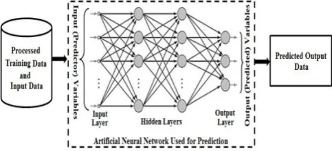
[image:1.595.306.548.303.413.2]and optimize for the point of minimum of the error function. A variety of training algorithms have been developed to search for the point of minimum error with their own plus and minus and here we compare the performance of gradient descent algorithm with scaled conjugate gradient algorithm based on supervised learning, by creating and experimenting with the prediction models employing data sets from life insurance sector.
Fig. 1. Prediction modeling based on artificial neural network.
II.REVIEW OF LITERATURE AND BACKGROUND MOTIVATION Gradient descent is a first order error optimization method for training of neural networks based prediction models and several attempts have been proposed to improve the efficiency of the method. Unfortunately, even for mildly nonlinear problems, this method shows a poor convergence and is not useful for such kind of practical applications [1]. Instead, more powerful methods such as Quasi–Newton [2]– [4] and conjugate gradient techniques are frequently preferred for training of the network in nonlinear cases. Use of second order derivative methods to improve the convergence speed is done because these methods show faster learning speeds in comparison to the methods, which only use first order gradient descent technique [5].
On the other hand, Newton's method converges much faster towards a local maximum or minimum than gradient descent, because it is second order optimization method [6] and approximates the second order terms of Taylor’s expansion as hessian matrix [7]. Newton's method uses curvature information to take a more direct route toward minimum. But computation of hessian is a big problem in these methods [8], [9], when there are more predictor variables and network is large in size or large weight vector.
A modification over Newton's method, Gauss–Newton method is to minimize a sum of squared function values and has the advantage that challenging computation of second order derivatives is not required. But, the main shortcoming
Improved Training of Predictive ANN with
Gradient Techniques
Dharminder Kumar,
Member, IAENG,
Sangeeta Gupta,
Member, IAENG
and Parveen Sehgal,
Member, IAENG
of Gauss–Newton based deterministic method is that the convergence to the global minima is not assured and also the estimation results strongly depend upon the initial choice of the input variables.
Levenberg Marquardt Algorithm (LMA) provides a numerical solution to the problem of minimizing the error function, which is generally nonlinear in nature. LMA actually interpolates [10] between Gauss–Newton Algorithm (GNA) and the method of gradient descent and is considered a trust region modification to Gauss–Newton Algorithm [11]. LMA is more robust than the GNA, because in many cases, it finds a solution even if its starting point is very far off the final minimum.
The chief advantage of Quasi–Newton methods is that the hessian matrix of second derivatives need not be evaluated directly but an approximation for the hessian is computed [12], [13], which is specified by approximate error energy gradient evaluation. But, on the negative side, Quasi– Newton algorithm requires more computation per iteration and more storage than the conjugate gradient methods, although it generally converges in less number of iterations. When weight dimension is large then conjugate gradient algorithm (CGM) is preferable to Quasi–Newton methods in computational terms [14].
The conjugate gradient algorithm [15] moves toward the point of minima using the error gradient and moving along successive noninterfering directions. It makes use of a line search method to compute the optimal step size along a line in the search direction to jump accurately inside valley of error surface. The line search bypasses the need to calculate the hessian matrix of second derivatives, but it requires computing the error at a number of points along the line. Computation of scalar β, which defines the relationship between noninterfering directions and selects the next search direction, is possible in several ways like Hestenes and Stiefel variation [16], Fletcher and Reeves variation [17], Daniel variation [18], Polak and Ribiere variation [19], [20] and some new variations like Dai and Yuan variation [21] and Hager and Zhang variation [22]. The direction of error minimization is always chosen such that the minimization steps in all previous directions are not spoiled [23]. The conjugate gradient methods consume comparatively less memory for large data size problems but they usually converge much more slowly than Newton or Quasi–Newton methods and require more number of iterations each time to find the next acceptable step. The method of conjugate gradients provides an effective way to optimize large, deterministic systems; however, it is not amenable to stochastic settings and tends to diverge.
The scaled conjugate gradient method bypasses the time consuming line search along conjugate directions [24], [25] and is considered to be the fastest one among the well known algorithms and in comparison to gradient decent algorithm for larger networks. When viewed as LMA, this method controls the indefiniteness in computation of second order hessian with help of a scalar parameter. It suppresses the instability by combining the trust region approach from the LMA with the CGM approach. This enables scaled conjugate gradient method to calculate the optimal step size in the selected search direction without complex and
expensive computation of line search used by the traditional conjugate gradient algorithms. But, there is a cost involved in estimation of the second order derivatives.
III. TECHNIQUES EMPLOYED FOR TRAINING THE NETWORK A. Gradient (Steepest) descent method
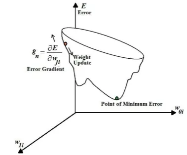
[image:2.595.331.521.237.394.2]In this method, we move near to the point of minimum error in small steps on the multidimensional error surface, in a direction opposite of the error gradient to search for the point of minima on the error surface [26]. It is shown in the Fig. 2. for a three dimensional error surface and it is difficult to visualize the error surface for higher dimensions.
Fig. 2. A cross-section of three dimensional error surface in employing gradient descent method for weight update in training of the network.
If we train our prediction model for N number of data points for the given data set and use error back propagation [27], [28] as supervised method for learning of the network, then overall training error present in the output layer for the nth data point is calculated as:
jD nj n
j
O
T
E
12 (
)
2 (1)Where, dataset D comprises of all the output neurons present in the output layer of the network model. For nthdata point of the employed data set,
T
jn represents desired target output andO
jn represents actual observed output from the designed system, for the jth output neuron in the output layer. Now, the gradient of overall error energy for nth data point i.e. changes of error energy w. r. t. weight values can be calculated as:ji n
w
E
g
Where,
w
ji represents the synaptic weights from the ith neuron in the previous hidden layer to the jth neuron in the output layer.ji j j ji n
w
O
O
E
w
E
g
.
(2)Now, from (1), we can say that:
)
(
j jj
O
T
O
E
(3)Also, in a multilayer perceptron neural network, output of any neuron present in the output layer is written as:
i i ji
j
w
I
O
, thereforei i i ji ji ji j
I
I
w
w
w
O
(4)Here,
I
i represents the input from i thneuron in previous layer. Now, using (2), (3) and (4), we can write:
i j j ji
n
T
O
I
w
E
g
(
)
(5)In order to move towards point of minimum error, a corrective weight adjustment must be applied in the reverse direction of error gradient, therefore, we can write:
i j j
ji
T
O
I
w
(
)
And thus, next updated values of the synaptic weights are computed in terms of previous weight values as:
ji ji
ji
w
w
w
prev
next
(6)Equation (6) is rewritten as (7), by introducing a control parameter
. i j j jiji
w
T
O
I
w
prev
next
(
)
(7)The learning rate parameter
regulates the speed at which we move toward the point of minimum error on the error surface and decides for the rate at which the network learns. Also performance of gradient descent is dependent upon type of back propagation used like incremental back propagation (IBP), batch back propagation (BBP) or Quick Propagation (QP) [29].B. Scaled conjugate gradient method
When computing the error energy for the next iteration, the scaled conjugate gradient method computes a numerical estimate close to the second order derivatives, instead of computing complex hessian matrix. In the kth iteration, a new search direction
d
k and a new step size
k are calculated to find the new values for the weight vector for the network,such that:
)
(
)
(
W
k kd
kE
W
kE
The quadratic approximation to
E
(
W
k)
in a neighbourhood of a pointW
k is given by the Taylor’s expansion [30]:z
W
E
z
z
W
E
W
E
z
W
E
(
k
)
(
k)
(
k)
T
21 T
(
k)
Since it is time consuming and takes more memory to compute the hessian
E
(
W
k)
therefore, second order informationO
k in terms of error gradient is approximated and computed as:k k k k k k k k
W
E
d
W
E
d
W
E
O
)
(
)
(
)
(
for1
0
k
Where,
E
(
W
k)
is the overall error energy in employing supervised learning,W
k denotes the weight vector for kth iteration,E
(
W
k)
is the gradient of error energy. The parameter
k sets the incremental change in the weight vector for the second derivative approximation.In this method, the trust region case of Levenberg Marquardt Algorithmis applied with the conjugate gradient approach to compute for the next step size. A new control variable
c
k is introduced to regulate the indefiniteness ofE
(
W
k)
. This is done by setting:k k k k k k k
k
c
d
W
E
d
W
E
O
)
(
)
(
And side by side we keep on computing
k
d
kTO
k for checking the indefiniteness ofE
(
W
k)
.In each iteration, we keep on adjusting
c
k, looking at the sign of
k, and it shows that hessianE
(
W
k)
is notpositive definite. If
k
0
thenc
k is slightly increased andO
k is computed again.Every time, the updated weight vector is computed as:
k k k
k
W
d
W
1
IV. EXPERIMENTAL OUTCOMES
Data sets of very large size, extracted from the running data warehouse in life insurance sector are used for training and testing of the prediction models for life insurance. These models based on the error back propagation technique with various error minimization learning algorithms under consideration are experimented with variety of model configurations with changed values of network parameters. The output variable, type of policy taken by the customer, is approximated for a set of input predictor variables like customers’ age, area and occupation of policy holders. The simulations are developed and tested in MathWorks MATLAB software and IBM SPSS software. Training
performance, error gradient and time taken to converge for minimum gradient values are observed to check for the efficiency of algorithms.
For developing all prediction models, we have simulated neural networks with tan–sigmoid transfer function at the hidden layer for normalizing the data signal coming from previous layers. We have tried a variety of configurations for the neural network with number of neurons in the hidden layer varying from 10 to 50. But 15 neurons in the hidden layer seem to be the optimal configuration for the data set and training methods under consideration.
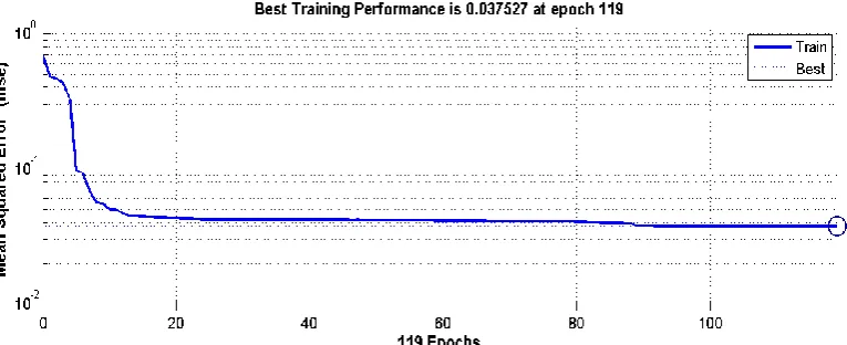
[image:4.595.112.486.234.394.2]Plots of training performance for different training methods, showing variation of mean square error verses numbers of epochs are shown in Fig. 3. to Fig. 5. as follows:
[image:4.595.107.488.419.575.2]Fig. 3. Training performance plot when employing gradient descent method
Fig. 4. Training performance plot when employing conjugate gradient method
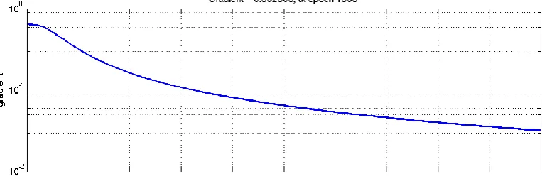
[image:4.595.107.490.599.755.2]The error gradient plots, employing different training methods are shown in Fig. 6. to Fig. 8. These graphs show the variation of error gradient with number of epochs. These plots also show the initial and final values of the gradients. It has been observed that gradient decent was unable to accomplish the target value of 0.0001 even in the 1000th epoch and on the other hand conjugate gradient method achieved the target in 135 epochs but the best and fastest
output was accomplished with the scaled conjugate gradient training function in 119 epochs, showing excellent accuracy in minimum time of convergence.
[image:5.595.106.488.167.293.2]We have developed a total of 66 simulations for prediction models of life insurance in MATLAB and 9 are developed in SPSS. The training results obtained with MATLAB for different training methods are as shown in Table I, which are the best performance values.
[image:5.595.111.490.340.465.2]Fig. 6. Gradient plot when employing gradient descent method
Fig. 7. Gradient plot when employing conjugate gradient method
Fig. 8. Gradient plot when employing scaled conjugate gradient method
TABLE I
SUMMARY OF OPTIMAL RESULTS WHEN EMPLOYING DIFFERENT TRAINING METHODS
Training Method
Hidden Layer Neurons
Minimum Gradient
Transfer Function
Final Epochs
Training Time
Training Performance
Initial Gradient
Final Gradient
Gradient Descent 15 0.0001 TANSIG 1000 0:16:14 0.0566 0.646 3.20E-02 Conjugate Gradient 15 0.0001 TANSIG 135 0:07:24 0.039 0.676 6.96E-05 Scaled Conjugate Gradient 15 0.0001 TANSIG 119 0:04:41 0.0375 0.447 8.04E-05
[image:5.595.108.490.514.651.2] [image:5.595.48.548.706.767.2]V.CONCLUSIONS AND FUTURE SCOPE
Training of neural network based prediction models, when applied to life insurance data, the scaled conjugate gradient method shows faster convergence in comparison with simple gradient descent and conjugate gradient methods. On an average, it shows approximately 3½ times faster convergence than simple gradient descent method toward minimum error. Moreover, our experiments indicate that gradient decent could train the models, maximum in the limits of order of 10-3, but scaled conjugate gradient was able to train the network to an accuracy level of the order of 10-4 and 10-5. Further, the results obtained by increasing the number of neurons in hidden layers from perceived optimal values only seem to increase the complexity of the network and don’t achieve any improvement in error correction.
However, analysis of problem can be extended in different angles like studying the effects of network parameters like number of neurons, hidden layers, learning rate and other network parameters etc. and drive mathematical formulations for optimal values of these parameters. Finding of new techniques and algorithms for more speedy training of the network model with faster convergence and prediction accuracy and guaranteed search for global minima in error surface are major works for future research.
ACKNOWLEDGMENT
We gratefully acknowledge KOTAK Life Insurance for providing the sample data sets for the research work and their valuable guidance in understanding the meaning of data.
REFERENCES
[1] J. C. Meza, “Steepest descent,” Wiley Interdiscip. Rev. Comput. Stat., vol. 2, no. 6, pp. 719-722, Dec. 2010.
[2] R. Fletcher, Practical Methods of Optimization. 2nd ed., vol. 1, John Wiley and Sons, 2000, ch. 3.
[3] J. A. Snyman, Practical Mathematical Optimization: An Introduction to Basic Optimization Theory and Classical and New Gradient-Based Algorithms. vol. 97, P. M. Pardalos, and D. W. Hearn, Ed. New York: Springer, 2005, ch. 2.
[4] S. S. Rao, Engineering Optimization Theory & Practice. 4th ed., New Jersey: John Wiley and Sons, 2009, ch. 6.
[5] E. Castillo, B. G. Berdinas, O. F. Romero, and A. A. Betanzos, “A very fast learning method for neural networks based on sensitivity analysis,” J. Mach. Learn. Res., Vol. 7, pp. 1159–1182, Jul. 2006. [6] S. Osowski, P. Bojarczak and M. Stodolski, “Fast second order
learning algorithm for feed forward multilayer neural networks and its applications,” Neural Netw., Elsevier, vol. 9, issue 9, pp. 1583–1596, Dec. 1996.
[7] R. Battiti, “First and second order methods for learning: between steepest descent and newton’s method,” Neural Comput., vol. 4, no. 2, pp. 141-166, Mar. 1992.
[8] W. L. Buntine, and A. S. Weigend, “Computing second derivatives in feed-forward networks: a review,” IEEE Trans. Neural Netw., vol. 5, no. 3, pp. 480–488, May. 1994.
[9] Raul Rojas, Neural Networks: A Systematic Introduction. Berlin: Springer, 1996, ch. 8.
[10] D. Marquardt, “An algorithm for least squares estimation of nonlinear parameters,” SIAM J. Appl. Math., vol. 11, no. 2, pp. 431-441, Jun. 1963.
[11] M. T. Hagan, and M. B. Menhaj, “Training feed forward networks with the marquardt algorithm,” IEEE Trans. Neural Netw., vol. 5, no. 6, pp. 989-993, Nov. 1994.
[12] A. Likas, and A. Stafylopatis, “Training the random neural network using quasi–newton methods,” Eur J. Oper. Res., Elsevier, vol. 126, issue 2, pp. 331-339, Oct. 2000.
[13] S. M. A. Burney, T. A. Jilani and C. Ardil, “A comparison of first and second order training algorithms for artificial neural networks,” Int. J. Comput. Intell., vol. 1, no. 3, pp. 176-182, Summer 2005.
[14] S. Haykin, Neural Networks: A Comprehensive Foundation. 2nd ed., Prentice Hall of India, 2008, pp.234-245.
[15] E. K. P. Chong, and S. H. Zak, An Introduction to Optimization. 2nd Ed., John Wiley and Sons, 2001, pp. 151-164.
[16] M. R. Hestenes, and E. Stiefel, “Methods of conjugate gradients for solving linear equations,” J. Res. Natl. Bur. Stand., vol. 49, no. 6, pp. 409–436, Dec. 1952.
[17] R. Fletcher, and C. Reeves, “Function minimization by conjugate gradients,” The Comput. J., vol. 7, issue 2, pp. 149-154, 1964. [18] J. W. Daniel, “The conjugate gradient method for linear and
nonlinear operator equations,” SIAM J. Numer. Anal., vol. 4, no. 1, pp. 10-26, Mar. 1967.
[19] E. Polak, and G. Ribiere, “Note on the convergence of methods of conjugate directions,” “Note sur la convergence de méthodes de directions conjuguées,” ESAIM: Mathematical Modelling and Numerical Analysis, vol. 3, issue: 1, pp. 35-43, 1969.
[20] E. Soria, J. D. Martin, and P. J. G. Lisboa, “Classical training methods,” in Metaheuristic procedures for training Neural Networks, E. Alba and R. Marti Ed., New York: Springer, 2006, pp. 25-32.
[21] Y. H. Dai, and Y. Yuan, “A nonlinear conjugate gradient method with a strong global convergence property,” SIAM J. Optim., vol. 10, issue 1, pp. 177 – 182, Jun. 1999.
[22] W. W. Hager, and H. Zhang, “A new conjugate gradient method with guaranteed descent and an efficient line search,” SIAM J. Optim., vol. 16, no. 1, pp. 170–192, Sep. 2005.
[23] P.P.v.d. Smagt, “Minimization methods for training feed forward neural networks,” Neural Netw., Elsevier, vol. 7, pp. 1-11, 1994. [24] M. F. Møller, “A scaled conjugate gradient algorithm for fast
supervised learning,” Neural Netw., Elsevier, vol. 6, issue 4, pp.525– 533, 1993.
[25] J. Lund´en, and V. Koivunen, “Scaled conjugate gradient method for radar pulse modulation estimation,” in Proc. IEEE Int. Conf. Acoust. Speech Signal Process. (ICASSP), Honolulu, Hawaii, 2007, vol. 2, pp. 297–300.
[26] M. T. Hagan, H. B. Demuth, and M. Beale, Neural Network Design. Boston: PWS Publishing, Reprint China Machine Press, 1996, pp. 9.2-9.5.
[27] E. Rumelhart, G. E. Hinton, and R. J. Williams, “Learning representations by back-propagating errors,” Nature, vol. 323, pp. 533-536, Oct. 1986.
[28] J. M. Nazzal, I. M. El-Emary and S. A. Najim, “Multilayer Perceptron Neural Network (MLPs) For Analyzing the Properties of Jordan Oil Shale,” World Appl. Sci. J., IDOSI Publications, vol. 5, no. 5, pp. 546-552, 2008.
[29] A. Ghaffari, H. Abdollahi, M. R. Khoshayand, I. S. Bozchalooi, A. Dadgar, and M. R. Tehrani, “Performance comparison of neural network training algorithms in modeling of bimodal drug delivery,” Int. J. Pharm., Elsevier, vol. 327, pp. 126-138, Aug. 2006.