Topological Optimization with the -Laplacian Operator and an Application in Image Processing

Volume 2009, Article ID 896813,20pages doi:10.1155/2009/896813

Research Article

Topological Optimization with the

p

-Laplacian

Operator and an Application in Image Processing

Alassane Sy

_{and Diaraf Seck}

1_{Universit´e de Bambey, Bambey, Senegal}

2_{Laboratoire de Math´ematique de la D´ecision et d’Analyse Num´erique (LMDAN), Ecole Doctorale de}

Math´ematiques et Informatique, Universit´e Cheikh Anta Diop de Dakar, B.p. 99 000 Dakar-Fann, Senegal

Correspondence should be addressed to Diaraf Seck,[email protected]

Received 14 April 2009; Revised 28 June 2009; Accepted 28 July 2009

Recommended by Kanishka Perera

We focus in this paper on the theoretical and numerical aspect os image processing. We consider a non linear boundary value problemthep-Laplacianfrom which we will derive the asymptotic expansion of the Mumford-Shah functional. We give a theoretical expression of the topological gradient as well as a numerical confirmation of the result in the restoration and segmentation of images.

Copyrightq2009 A. Sy and D. Seck. This is an open access article distributed under the Creative Commons Attribution License, which permits unrestricted use, distribution, and reproduction in any medium, provided the original work is properly cited.

1. Introduction

The goal of the topological optimization problem is to find an optimal design with an a priori poor information on the optimal shape of the structure. The shape optimization problem consists in minimizing a functionaljΩ JΩ, uΩ where the functionuΩ is defined, for

example, on a variable open and bounded subsetΩofRN.Forε >0,letΩε Ω\x0εω

be the set obtained by removing a small partx0εωfromΩ,wherex0 ∈Ωandω ⊂ RN is

a fixed open and bounded subset containing the origin. Then, using general adjoint method, an asymptotic expansion of the function will be obtained in the following form:

jΩε jΩ fεgx0 o

fε,

lim

ε→0fε 0, fε>0.

1.1

The topological sensitivitygx0provides information when creating a small hole located at

In this paper, we study essentially a topological optimization problem with a nonlinear operator. There are many works in literature concerning topological optimization. However, many of these authors study linear operators. We notice that Amstutz in1established some results in topological optimization with a semilinear operator of the form−Δuφu 0 in a domainΩwith some hypothesis inφ.

In this paper, we will limit in thep-Laplacian operator and we reline the theoretical result obtained with an application in image processing.

The paper is organized as follows: inSection 2, we recall image processing models and the Mumford-Shah functional which are widely studied in literature. InSection 3, we present the general adjoint method. Section 4 is devoted to the topological optimization problem and the main result of the paper which is proved inSection 5. InSection 6, the topological optimization algorithm and numerical applications in image processing are presented.

2. Formulation of the Problem

2.1. A Model of Image Processing

Many models and algorithms2have been proposed for the study of image processing. In3, Koenderink noticed that the convolution of signal with Gaussian noise at each scale is equivalent to the solution of the heat equation with the signal as initial datum. Denoting byu0this datum, the “scale space” analysis associated withu0 consists in solving

the system

∂ux, t

∂t Δux, t ux,0 u0x

inRN. 2.1

The solution of this equation with an initial datum is ux, t Gt ∗ u0, where Gσ

1/4πσexp−x2/4σis the Gauss function, andxthe euclidian norm ofx∈RN_.

In4, Malik and Perona in their theory introduced a filter in2.1for the detection of edges. They proposed to replace the heat equation by a nonlinear equation:

∂u ∂t div

f|∇u|∇u

ux,0 u0x

inRN. 2.2

Nordstr ¨om5introduced a new term in2.2which forcesux, tto remain close to x.Because of the forcing termu−v,the new equation

∂u ∂t −div

f|∇u|∇uv−u inΩ×0, T

∂u

∂ν 0 in ∂Ω×0, T ux,0 u0x inΩ× {t0}

2.3

has the advantage to have a nontrivial steady state, eliminating, therefore, the problem of choosing a stoping time.

2.2. The Mumford-Shah Functional

One of the most widely studied mathematical models in image processing and computer vision addresses both goals simultaneously, namely, Mumford and Shah6who presented the variational problem of minimizing a functional involving a piecewise smooth repre-sentation of an image. The Mumford-Shah model defines the segmentation problem as a joint smoothing/edge detection problem: given an imagevx,one seeks simultaneously a “piecewise smoothed image”uxwith a setKof abrupt discontinuities, the edges ofv. Then the “best” segmentation of a given image is obtained by minimizing the functional

Eu, K

Ω\K

α|∇u|2βu−v2dxHN−1K, 2.4

whereHN−1_{Kis theN−1-dimensional Hausdorffmeasure ofKandαandβare positive}

constants .

The first term imposes thatuis smooth outside the edges, the second that the piecewise smooth imageuxindeed approximatesvx,and the third that the discontinuity setKhas minimal lengthand, therefore, in particular, it is as smooth as possible.

The existence of minimums of the Mumford-Shah has been proved in some sense, we refer to7. However, we are not aware that the existence problem of the solution for this problem is closed.

Before beginning the study of the topological optimization method, let us recall additional information about the other techniques.

We say that an image can be viewed as a piecewise smooth function and edges can be considered as a set of singularities.

We recall that a classical way to restore an imageufrom its noisy versionvdefined in a domain included inR2_{is to solve the following PDE problem:}

u−divc∇u v inΩ,

∂u

∂ν 0 in∂Ω,

wherecis a small positive constant. This method is well known to give poor results: it blurs important structures like edges. In order to improve this method, nonlinear isotropic and anisotropic methods were introduced, we can cite here the work of Malik and Perona, Catt´e et al., and, more recently, Weickert and Aubert.

In topological gradient approach,ctakes only two values:c0, for example,c01, in the

smooth part of the image and a small valueon edges. For this reason, classical nonlinear diffusive approaches, where c takes all the values of the interval , c0,could be seen as

a relaxation of the topological optimization method. Many classification models have been studied and tested on synthetic and real images in image processing literature, and results are more or less comparative taking in to account the complexity of algorithms suggested and/or the cost of operations defined. We can cite here some models enough used like the structural approach by regions growth, the stochastic approaches, and the variational approaches which are based on various strategies like level set formulations, the Mumford-Shah functional, active contours and geodesic active contour methods, or wavelet transforms.

The segmentation problem consists in splitting an image into its constituent parts. Many approaches have been studied. We can cite here some variational approaches such as the use of the Mumford-Shah functional, or active contours and snakes. Our approach consists in using the restoration algorithm in order to find the edges of the image, and we will give a numerical result.

To end this section, let us sum up our aim about the numerical aspects.

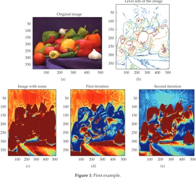
Considering the Mumford Shah functional, our objective in the numerical point of view is to apply topological gradient approach to images. We are going to show that it is possible to solve these image processing problems using topological optimization tools for the detection of edges the topological gradient method is able to denoise an image and preserve features such as edges. Then, the restoration becomes straightforward, and in most applications, a satisfying approximation of the optimal solution is reached at the first iteration or the second iteration of the optimization process.

We refer the reader, for additional details, to the work in8–17.

3. General Adjoint Method

In this section, we give an adaptation of the adjoint method introduced in18to a nonlinear problem. LetVbe a Hilbert space and let

aεu, v lεv, v∈ V, 3.1

be a variational formulation associated to a partial differential equation. We suppose that there exist formsδau, v, δl,and a functionfε>0 which goes to zero whenεgoes to zero. Letuεresp.,u0be the solution of3.1forε >0resp., forε0.

We suppose that the following hypothesis hold:

H-1uε−u0Vofε,

H-2aε−a0−fεδa_VOfε,

H-3lε−l0−fεδl_VOfε.

Letjε Jεuεbe the cost function. We suppose that forε 0, J0u0 Ju0is

H-4We suppose that there exists a functionδJsuch that

Jεuε−J0u0 DJu0uε−u0 fεδJu0 O

fε. 3.2

Under the aforementioned hypothesis, we have the following theorem.

Theorem 3.1. Letjε Jεuεbe the cost function, thenjhas the following asymptotic expansion:

jε−j0 δau0, w0 δJu0−δlw0fε o

fε, 3.3

wherew0is the unique solution of the adjoint problem: findw0such that

a0

φ, w0

−DJu0φ, ∀φ∈ V. 3.4

The expressiongx0 δaux0, ηx0δJux0−δlηx0is called the topological

gradient and will be used as descent direction in the optimization process.

The fundamental property of an adjoint technique is to provide the variation of a function with respect to a parameter by using a solutionu_Ω and adjoint statev_Ω which do not depend on the chosen parameter. Numerically, it means that only two systems must be solved to obtain the discrete approximation ofgxfor allx∈Ω.

Proof ofTheorem 3.1. LetLu, η au, η Ju−lηbe the Lagrangian of the system as introduced by Lions, in19and applied by Cea in optimal design problems in18. We use the fact that the variation of the Lagrangian is equal to the variation of the cost function:

jε−j0 Lε

uε, η

− L0

u0, η

aε

uε, η

−lε

η−a0

u0, η

−l0

η Jεuε−Ju0

aεuε, η−a0u, η

i

−lεη l0η

ii

Jεuε−Ju0

iii

.

3.5

It follows from hypothesisH-2thatiis equal to

aε

uε, η

−a0

u0, η

fεδau0, η

Ofε, 3.6

H-3implies thatiiis equal to

lε

η−l0

ηfεδlηOfε, 3.7

andH-4gives an equivalent expression ofiii

Jεuε−J0u0 DJu0uε−u0 fεδJu0 O

Further3.5becomes

jε−j0 fεδau0, η

δJu0−δl

ηDJu0uε−u0 O

fε. 3.9

Letη0be the solution of the adjoint problem: findη0∈ Vsuch that

a0

φ, η0

−DJu0φ, ∀φ∈ V. 3.10

It follows from the hypothesisH-1–H-4that

jε j0 fεgx0 O

fε, ∀x0∈Ω, 3.11

which finishes the proof of the theorem.

4. Position of the Problem and Topological Sensitivity

Initial domain Perturbed domain

Forε >0, letΩε Ω\ωε,whereωεx0εω0, x0∈Ω,andω0⊂RNis a reference domain.

The topological optimization problem consists of determining the asymptotic expansion of theN-dimensional part of the Mumford-Shah energy, and applying it to image processing. Forv∈L2_{Ω,let us consider the functional}

JΩεuε α

Ωε

|∇uε|2dxβ

Ωε

uε−v2dx, 4.1

whereuεis the solution of the stationary model of2.3withfs |s|p−2, p >1, that is,uε

satisfies

uε−div

|∇uε|p−2∇uε

v inΩε,

∂uε

∂ν 0 on ∂Ωε\∂ωε, uε0 on ∂ωε,

α, βare positive constants and forε0, u0uis the solution of

u−div|∇u|p−2∇uv inΩ,

∂u

∂ν 0 on ∂Ω∈L

2_Ω.

∈L2Ω 4.3

Before going on, let us underline that interesting works were done by Auroux and Masmoudi

10, Auroux et al. 12, and Auroux11by considering the Laplace operator, that is,p2 and the first term of the Mumford Shah functional, that is,

JΩu

Ω|∇u|

2_{d, 4.4}

as criteria to be optimized.

Contrarily to the Dirichlet case, we do not get a natural prolongment for the Neumann condition to the boundary ∂Ω. For this reason, all the domains which will be used are supposed to satisfy the following uniform extension propertyP.LetDbe an open subset ofRN_:

P

⎧ ⎪ ⎪ ⎪ ⎪ ⎪ ⎪ ⎪ ⎨ ⎪ ⎪ ⎪ ⎪ ⎪ ⎪ ⎪ ⎩

i ∀ω⊂D, there exist a continuous and linear operator

of prolongment Pω : W1,pω−→W1,pDand apositive constant

cω such thatPωuW1,p_D≤cω uW1,p_ω,

ii there exists aconstant M >0 such that∀ω⊂D, Pω ≤M.

4.5

Lemma 4.1. Letv∈L2_{Ωproblem4.3(resp.,4.2) has a unique solution. Moreover, one has}

uε−u0VOfε, 4.6

where

u_Vu_L2_Ω∇u_Lp_Ω

Ω|u|

2_dx 1/2

Ω|∇u| p_dx

1/p

. 4.7

In order to prove the lemma, we need the following result which in20, Theorem 2.1. LetΩbe a bounded open domain ofRN_{no smoothness is assumed on∂Ωandp, pbe real}

numbers such that

1< p, p<∞, 1 p

1

p 1. 4.8

Consider the operatorAdefined onW1,p_Ωby

wherea:Ω×R×RN _{→ Ris a Caratheodory function satisfying the classical Laray-Lions}

hypothesis in the sense of20, described in what follows:

|ax, s, ζ| ≤cx k1|s|p−1k2|ζ|p−1, 4.10

ax, s, ζ−ax, s, ζ∗ζ−ζ∗>0, 4.11

ax, s, ζζ

|ζ||ζ|p−1 −→|ζ| →∞∞ , 4.12

almost everyx∈Ω, for alls∈R, ζ, ζ∗∈RN_{, ζ /ζ}∗_.

Consider the nonlinear elliptic equation

−divax, un,∇un fngn inDΩ. 4.13

We assume that

un converges touonW1,pΩweakly and strongly inLp_locΩ, 4.14

fn−→f strongly inW−1,p

Ω, and almost everywhere inΩ. 4.15

The hypotheses 4.13–4.15 imply that gn ∈ W−1,p

Ω and is bounded on this set. We suppose eithergnis bounded inMbΩ space on Radon measures, that is,

_{gn, ϕ≤cKϕ}

L∞_K, ∀ϕ∈ DK, with supp

ϕ⊂K, 4.16

cKis a constant which depends only on the compactK.

Theorem 4.2. If the hypotheses4.10–4.15are satisfied, then

∇un−→ ∇u strongly in

Lm_locΩN, ∀m < p, 4.17

whereuis the solution of

−divax, u,∇u fg in DΩ. 4.18

For the proof of the theorem, we refer to20.

Remark 4.3. Such assumptions are satisfied if ax, s, ζ |ζ|p−2_{ζ, that is, the operator with}

Proof ofLemma 4.1.We prove at first that4.3has a unique solution. The approach is classic: the variational approach.

Let

Vu∈L2Ω,∇u∈LpΩN, andusatisfying the propertyP, 4.19

Iu 1 2

Ωu

2_dx 1

p

Ω|∇u| p_dx−

Ωu·vdx. 4.20

If there existsu ∈ Vsuch thatIu minη∈VIη, then usatisfies an optimality condition

which is the Euler-Lagrange equationIu 0.Leth∈ DΩ, t∈R,

Iuth 1 2

Ωuth

2_dx1

p

Ω|∇uth|

p_dx−

Ωvuthdx

1

2

Ωuth

2_dx1

p

Ω

|∇uth|2p/2dx−

Ωvuthdx

1

2

Ωuth

2_dx1

p

Ω

|∇u|22t∇u∇ht2_|∇h|2p/2_dx

−

Ωvuthdx.

4.21

Using Taylor expansion, it follows that

Ω

|∇u|pt∇h∇u|∇u|p−2−uv−thvdxot,

Iu, hlim

t→0

Iuth−Iu

t 0⇐⇒

u−div|∇u|p−2∇u−v, h0, ∀h∈ DΩ.

4.22

Sinceh∈ DΩ,we haveu−div|∇w|p−2∇u vinDΩ.

Now, let u ∈ W1,p_{Ω be a weak solution of 4.3, then the variational formulation}

gives

Ω

uϕ|∇u|p−2∇u∇ϕ−

Γ|∇u| p−2∂u

∂ν

Ωvϕ. 4.23

Let us introduceC1

cΩbe the set of functionsC1-regular inΩand with compact support in

Ω.Choosingϕ∈C1

cΩ, it follows that

We come back to4.3withϕ∈C1_{Ω, and we obtain}

∂Ω|∇u| p−2∂u

∂νϕ0, 4.25

asuis not constant almost everywhere, we obtain

∂u

∂ν 0 on∂Ω. 4.26

Consequently4.3admits a unique solution which is obtained by minimizing the functional

4.20. For achieving this part of the proof, it suffices to prove that the problem: findu ∈ V such that

Iu min

η∈V I

η _4.27

admits a unique solution, whereI·is defined by4.20.

In fact,Iwis a strict convex functional and the setVis convex. To achieve our aim, we prove thatI·is bounded from what follows: letαinfη∈VIη,thenα >−∞.

We have

Iη≥ 1 2

Ωη

2_dx−

Ωη·vdx≥

1 2η

2

L2_Ω− v_L2_Ωη_L2_Ω

≥Ev 2

L2_Ω

>−∞,

4.28

whereEX X2_{− v}

L2_ΩX.

This proves thatI·has a unique minimum and this minimum is the solution of4.3. We use the same arguments to prove that 4.2 admits a unique solution and the solution is obtained by minimizing the functional4.1in the set

Vε

u∈L2Ω, ∇u∈LpΩN, usatisfiesP, u0 on∂ωε

. 4.29

To end the proof, we have to prove that||uε−u0||V → 0

ε→0.

On the one hand, we suppose for simplicity thatωεBx0, ε.The proof will remain

true if ωε is regular enough, for example,∂ωε has a Lipschitz regularity with a uniform

Lipschitz’s constant. Letε 1/n,here and in the following, we setun uε uΩn.That

is,unis the solution of

un−div

|∇un|p−2∇un

v in Ωn,

∂un

∂ν 0 on∂Ω ∂Ωn\∂B

x0,

1 n

,

un0 on∂B

x0,

1 n

.

Letunbe the extension ofuεinBx0,1/n, that is,

unx

⎧ ⎪ ⎪ ⎨ ⎪ ⎪ ⎩

unx, ifx∈Ωn,

0, ifx∈B

x0,

1 n

.

4.31

The variational form of the problem is

Ωu

2

ndx

Ω|∇un|

p_dx

Ωunvdx. 4.32

Since

|∇un|p≥0, we get

Ω|∇un|

p_{dx≥0. 4.33}

This implies that

Ω|un|

2_dx≤

Ω|unv|dx. 4.34

By Cauchy-Schwarz inequality, we have

un2L2_Ω≤ unL2_Ωv_L2_Ω, 4.35

and then

unL2_Ω≤ v_L2_Ω≤c₁. 4.36

By the same arguments, and estimation4.36, we prove that

∇unLp_Ω≤ v_L2_Ω≤c2. 4.37

SinceΩis bounded,unL2_Ωand∇unLp_Ωare bounded, and thus there existu∗ ∈L2Ω

andT ∈Lp_ΩN_{such that}

un

σL2_,L2u

∗_{, ∇u}

n

σLp_,LpT, 4.38

we can prove now thatT ∇u∗almost everywhere inΩ:

∂un

∂xi σLp_,LpTi i1, . . . , N

⇐⇒ ∀f∈LpΩ,

∂un

∂xi

, f

−→T, f,

DΩ⊂Lp_{Ω,thus for allϕ∈ DΩ,}

Ti, ϕ

←−

∂un

∂xi, ϕ

−

un,

∂ϕ ∂xi

−→ −

u∗, ∂ϕ ∂xi

. 4.40

Thus,

T, ϕ−

u∗, ∂ϕ ∂xi

, ∀ϕ∈ DΩ,

⇒Ti

∂u∗ ∂xi inD

_{Ω ⇒T}

i

∂u∗

∂xi almost everywhere inΩ.

4.41

It follows from4.38thatun σL2_,L2u

∗_{andϕ∈ DΩthus∂ϕ/∂x}

i∈ DΩ. This implies that

−

un,

∂ϕ ∂xi

−→ −

u∗, ∂ϕ ∂xi ∂u∗ ∂xi , ϕ , ∂u∗ ∂xi , ϕ

T, ϕ, ∀ϕ∈ DΩ ⇒Ti

∂u∗ ∂xi

almost everywhere.

4.42

Thus it follows from the Theorem 4.2that u∗ u, and ∇u ∇u∗, and we deduce ||un −

u∗||_V.

The main result is the following which gives the asymptotic expansion of the cost function.

Theorem 4.4Theoremmain result. Letjε Jεuεbe the Mumford-Shah functional. Then

jhas the following asymptotic expansion:

jε−j0 fεδju0, η0

ofε, 4.43

whereδju0, η0 δau0, η0 δJu0−δlη0andη0is the unique solution of the so-called adjoint problem: findη0such that

a0

ψ, η0

−DJu0ψ ∀ψ∈ V. 4.44

5. Proof of the Main Result

A sufficient condition to prove the main result is to show at first that the hypothesisH-1,

H-2,H-3, andH-4 cf.Section 3are satisfied. Then we apply in the second step of the proof theTheorem 3.1to get the desired result.

TheLemma 4.1gives the hypothesisH-3. The variational formulation associated to3.1is

Ωε

uεφdx

Ωε

|∇uε|p−1∇uε∇φdx

Ωε

We set

aε

uε, φ

Ωε

uεφdx

Ωε

|∇uε|p−1∇uε∇φdx, ∀φ∈ Vε,

lε

φ

Ωε

vφdx, ∀φ∈ Vε.

5.2

5.1. Variation of

aε

−

a

Proposition 5.1. The asymptotic expansion ofaεis given by

aε

uε, η

−a0

u, η−fεδau, ηOfε, 5.3

where

fεδau, η−

ωε

uη|∇u|p−2∇u∇ηdx

!

, ∀η∈ Vε. 5.4

For the proof, we need the following result:

Theorem 5.2TheoremEgoroff’s theorem. Letμbe a measure onRN_{and supposef}

k:RN →

Rm_{k 1,2, . . .areμ-measurable. Assume alsoA ⊂ R}N _{is μ-measurable, with μA < ∞,and}

fk → gμa.e onA. Then for each >0there exists aμ-measurable setB⊂Asuch that

iμA−B< ,

iifk → guniformly onB.

For the proof of Egoroff’s theorem we refer to21.

Proof ofProposition 5.1.

aε

uε, η

−a0

u, η

Ωε

uεηdx

Ωε

|∇uε|p−2∇uε∇ηdx

−

Ωuηdx−

Ω|∇u|

p−2_∇u∇ηdx

Ωε

uε−uηdx

I

Ωε

|∇uε|p−2∇uε− |∇u|p−2∇u∇ηdx

II

−

ωε

uη|∇u|p−2∇u∇ηdx

We have now to prove that I and II tend to zero withε. Estimation of I:

Ωε

uε−uηdx

≤

"

Ωε

η2dx

#1/2"

Ωε

|uε−u|2dx

#1/2

≤

Ωη

2_dx 1/2

Ω|uε−u|

2_dx 1/2

becauseΩε⊂Ω

uε−uL2_Ωη_L2_Ω.

5.6

As||uε−u||L2_Ω ≤ ||u_ε−u||_V Ofε cf.Lemma 4.1, it follows that

$

Ωεuε−uηdx → 0

withfε.

Estimation of II:

Ωε

|∇uε|p−2∇uε− |∇u|p−2∇u

∇wdx ≤ Ω

|∇uε|p−2∇uε− |∇u|p−2∇u

∇wdx. 5.7

Letε1/nandgn |∇un|p−2∇un− |∇u|p−2∇u∇w,thengn converges almost every where

to zero, by usingLemma 4.1. Writing

Ωgndx

A0 gndx

Ac

0

gndx≤ lim n→∞sup_x∈A

0

gn

Ac

0Ω\A0

gndx. 5.8

ifΩ\A0is negligible, then $

Ω\A0gndx0,and by using Egoroff’s theorem, we obtain that II goes to zero.

Otherwise, we iterate the operation untilk0,such thatΩ\%k_i0₀Aibe a set of zero

measure. Then we get

Ωgndx

∪k₀ i0Ai

gndx

Ω\∪k₀ i0Ai

gndx. 5.9

AsΩ\%k0

i0Aiis a set of zero measure, the second part of this equation is equal to zero,

and we conclude by using Egoroff’s theorem that$_Ωgndxgoes to zero, because%k_i0₀Ai is

measurable. It follows that II goes to zero. We set now

fεδau, η−

ωε

uη|∇u|p−1∇u∇ηdx 5.10

5.2. Variation of the Linear Form

Proposition 5.3. The variation of the linear formlεis given by

lε

η−l0

η−fεδlη0, 5.11

where

fεδlu, η−

ωε

vηdx, ∀η∈ Vε. 5.12

5.3. Variation of the Cost Function

In this section, we will prove that the cost function satisfies the necessary condition for applying theTheorem 3.1hypothesisH-4.

Proposition 5.4. LetJ0ube the Mumford-Shah functional

Ju α

Ω|∇u|

2_dxβ

Ω|u−v|

2_{dx, 5.13}

Jhas the following asymptotic expansion:

Jεuε−J0u0 DJεu0uε−u0 fεδJu0 o

fε. 5.14

Proof. It holds that

Jεuε−Ju0

Ωε

α|∇uε|2dx

Ωε

β|uε−v|2dx

−

Ωα|u0|

2_dx

Ωβ|u0−v|

2_dx

Ωε

α|∇uε|2− |∇u0|2

dx

Ωε

β|uε−v|2− |u0−v|2

dx

− "

ωε

α|∇u0|2dx

ωε

β|u0−v|2dx #

,

Ωε

α|∇uε|2− |∇u0|2

dx

Ωε

α|∇uε−u0|2

dx2α

Ωε

∇u0· ∇uε−u0dx.

Due to the fact thatuε u0|Ωε, it suffices to evaluate the differenceJε−J0inDεwhereDε

Bx0, R\ωε, andωε ⊂Bx0, R⊂Ω. TakingLemma 4.1, we haveuε−u0V ofε,one

only needs to prove that

Dε

|∇uε−u0|2dxo

fε,

Dε

|∇uε−u0|2dx≤

Bx0,R

|∇uε−u0|2dx

≤measBx0, Rp−2/p∇uε−u02Lp_Ω

≤measBx0, Rp−2/puε−u02_V.

5.16

The same arguments as above yield

Dε

β|uε−v|2− |u0−v|2

dx

Dε

β|uε−u0|2dx

Dε

2βv−u0uε−u0dx, 5.17

Dε

β|uε−u0|2dx≤

Ωβ|uε−u0|

2_{dx≤βmeasΩ}

uε−u0_V. 5.18

Lemma 4.1proves thatuε−u0_Vofε,this implies that

Dε

β|uε−u0|2dxo

fε. 5.19

Let us set

DJu0η

Dε

2βv−u0ηdx2α

Dε

∇u0· ∇ηdx; ∀η∈ Vε, 5.20

then we obtain

Jεuε−J0u0 DJu0uε−u0 fεδJu0 o

fε 5.21

with

fεδJu0 −

ωε

α|∇u0|2dx

ωε

β|u0−v|2dx !

. 5.22

Hence, the hypothesis H-1–H-4 are satisfied, and it follows from the

Theorem 3.1that

jε j0 fεgx0 o

50 100 150 200 250 300 350

100 200 300 400 500 Original image

a

50 100 150 200 250 300 350

100 200 300 400 500 Level sets of the image

b

50 100 150 200 250 300 350

100 200 300 400 500 Image with noise

c

50 100 150 200 250 300 350

100 200 300 400 500 First iteration

d

50 100 150 200 250 300 350

100 200 300 400 500 Second iteration

e

Figure 1:First example.

where

gx0 δa

u0, η0

δJu0−δl

η0

, 5.24

which finishes the proof ofTheorem 4.2.

6. Numerical Results

Remark 6.1. In the particular case wherep2 andωBx0,1, the problem becomes

minJu, Ju

Ωα|∇u|

2_dx

Ω|u−v|

100 200 300 400 500

100 200 300 Original image

a

100 200 300 400 500

100 200 300 Level sets of the image

b

100 200 300 400 500

100 200 300 Image with noise

c

100 200 300 400 500

100 200 300 First iteration

d

100 200 300 400 500

100 200 300 Second iteration

e

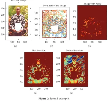
Figure 2:Second example.

whereuis the solution of

u−Δuv inΩ,

∂u

∂ν 0 on∂Ω.

6.2

The topological gradient is given by

gx0 −2π

α|∇ux0|2α∇ux0· ∇ηx0 β|ux0−vx0|2

, 6.3

whereηis the solution of the adjoint problem

η−Δη−DJu inΩ,

∂η

∂ν 0 on∂Ω.

50 100 150 200 250

50 100 150 200 250 Original image

a

50 100 150 200 250

50 100 150 200 250 Level set of the image

b

50 100 150 200 250

50 100 150 200 250 Image with noise

c

50 100 150 200 250

50 100 150 200 250 First iteration

d

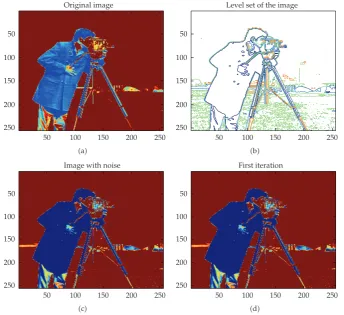
Figure 3:Third example.

6.1. Algorithm

1input: image with noise;

2computeuandwdirect state and adjoint stateby finite element method;

3compute the topological gradientg;

4drill a hole wheregis “most” negative;

5defineuεin the hole;

6if “stopping criteria” is not satisfied, goto 2 else stop.

6.2. Numerical Examples

References

1 S. Amstutz, “Topological sensitivity analysis for some nonlinear PDE system,” Journal de Math´ematiques Pures et Appliqu´ees, vol. 85, no. 4, pp. 540–557, 2006.

2 S. Masnou and J. M. Morel, “La formalisation math´ematique du traitement des images”. 3 J. J. Koenderink, “The structure of images,”Biological Cybernetics, vol. 50, no. 5, pp. 363–370, 1984. 4 J. Malik and P. Perona, “A scale-space and edge detection using anisotropic diffusion,” inProceedings

of IEEE Computer Society Worhshop on Computer Vision, 1987.

5 N. K. Nordstr¨aom,Variational edge detection, Ph.D. dissertation, Departement of Electrical Engineering, University of California at Berkeley, Berkeley, Calif, USA, 1990.

6 D. Mumford and J. Shah, “Optimal approximations by piecewise smooth functions and associated variational problems,”Communications on Pure and Applied Mathematics, vol. 42, no. 4, pp. 577–685, 1989.

7 J.-M. Morel and S. Solimini,Variational Methods in Image Segmentation, vol. 14 ofProgress in Nonlinear Differential Equations and Their Applications, Birkh¨auser, Boston, Mass, USA, 1995.

8 G. Aubert and J.-F. Aujol, “Optimal partitions, regularized solutions, and application to image classification,”Applicable Analysis, vol. 84, no. 1, pp. 15–35, 2005.

9 G. Aubert and P. Kornprobst,Mathematical Problems in Image Processing. Partial Differential Equations and the Calculus of Variations, vol. 147 ofApplied Mathematical Sciences, Springer, New York, NY, USA, 2001.

10 D. Auroux and M. Masmoudi, “Image processing by topological asymptotic expansion,”Journal of Mathematical Imaging and Vision, vol. 33, no. 2, pp. 122–134, 2009.

11 D. Auroux, “From restoration by topological gradient to medical image segmentation via an asymptotic expansion,”Mathematical and Computer Modelling, vol. 49, no. 11-12, pp. 2191–2205, 2009. 12 D. Auroux, M. Masmoudi, and L. Belaid, “Belaid image restoration and classification by topological

asymptotic expansion,” inVariational Formulations in Mechanics: Theory and Applications, E. Taroco, E. A. de Souza Neto, and A. A. Novotny, Eds., CIMNE, Barcelona, Spain, 2006.

13 N. Paragios and R. Deriche, “Geodesic active regions and level set methods for supervised texture segmentation,”International Journal of Computer Vision, vol. 46, no. 3, pp. 223–247, 2002.

14 J. Weickert, Anisotropic diffusion in image processing, Ph.D. thesis, University of Kaiserslautern, Kaiserslautern, Germany, 1996.

15 J. Weickert, “Efficient image segmentation using partial differential equations and morphology,”

Pattern Recognition, vol. 34, no. 9, pp. 1813–1824, 2001.

16 G. Aubert and L. Vese, “A variational method in image recovery,”SIAM Journal on Numerical Analysis, vol. 34, no. 5, pp. 1948–1979, 1997.

17 J.-F. Aujol, G. Aubert, and L. Blanc-F´eraud, “Wavelet-based level set evolution for classification of textured images,”IEEE Transactions on Image Processing, vol. 12, no. 12, pp. 1634–1641, 2003.

18 J. C´ea, “Conception optimale ou identification de formes: calcul rapide de la d´eriv´ee directionnelle de la fonction co ˆut,”RAIRO Mod´elisation Math´ematique et Analyse Num´erique, vol. 20, no. 3, pp. 371–402, 1986.

19 J.-L. Lions, Sur Quelques Questions d’Analyse, de M´ecanique et de Contrˆole Optimal, Les Presses de l’Universit´e de Montr´eal, Montreal, Canada, 1976.

20 L. Boccardo and F. Murat, “Almost everywhere convergence of the gradients of solutions to elliptic and parabolic equations,”Nonlinear Analysis: Theory, Methods & Applications, vol. 19, no. 6, pp. 581– 597, 1992.