Stochastic-Based Power Consumption Analysis for Data Transmission in Wireless Sensor Networks

Stochastic-Based

Power

Consumption

Analysis

for

Data

Transmission

in

Wireless

Sensor

Networks

Minh

T.

Nguyen

,

Hien

M.

Nguyen

,

Antonino

Masaracchia

,

Cuong

V.

Nguyen

2_{DuyTanUniversity,Vietnam} 3_{Queen’sUniversityBelfast,UK}

4_{UniversityofInformationandCommunicationTechnology,Vietnam}

Abstract

Wireless sensor networks (WSNs) provide a lot of emerging applications. They suffer from some limitations such as energy constraints and cooperative demands essential to perform sensing or data routing. The networks could be exploited more effectively if they are well managed with power consumption since all sensors are randomly deployed in sensing areas needed to be observed without battery recharge or remote control. In this work, we proposed some stochastic-based methods to calculate total power consumption for such networks. We model common arbitrary networks with different types of sensing areas, circular and square shapes, then analyze and calculate the power consumption for data transmission based on statistic problems. Almost common data collection methods are employed such as cluster-based, tree-based, neighborhood based and random routing. In each method, the total power consumption is formulated and then simulated to be verified. This paper shows promise that all the formulas could be applied not only on WSNs but also mobile sensor networks (MSNs) while the mobile sensors are considered moving at random positions.

Received on 05 June 2019; accepted on 12 June 2019; published on 13 June 2019

Keywords: Wireless sensor networks, data collection, clustering, random walk, routing tree, power consumption. Copyright © 2019 Minh T. Nguyen etal., licensed to EAI. This is an open access article distributed under the terms of the Creative Commons Attribution license (http://creativecommons.org/licenses/by/3.0/), which permits unlimited use, distribution and reproduction in any medium so long as the original work is properly cited.

doi:10.4108/eai.13-6-2019.159123

1. Introduction

Wireless Sensor networks (WSNs) generally are intended to monitor or detect events due to each specific application [1,2]. In the networks, sensors are often dropped and deployed randomly into sensing areas that need to be observed. The random positions of the sensors in the networks lead to difficulty of managing sensor energy that could disconnect such networks earlier than planed. The sensors connect to each other based on an appropriate transmission range or a broadcast information asking for connections due to routing algorithms [3]. The network topologies are predesigned or self-organized depending on their purposes. They are often tree-based, cluster-based or

H_{Corresponding author: Minh T. Nguyen} ([email protected]).

random routing algorithms that we will consider in this work for stochastic analysis.

different shapes of sensing areas, different assumptions and network models that provide flexible tools for calculating in WSNs.

The remainder of this paper is organized as follows. The background about power consumption for data transmission in general and related work are mentioned in Section II. Each data collection method is presented separately in each following section in which Random Walk Routing, Tree-Based Data Gathering, Cluster-Based and Neighborhood-Based Data Collection methods are addressed in Sections III, IV, V, VI, respectively. In each section, the power consumption for any data transmission in WSNs related to each data collection method is formulated, analyzed and simulated. Finally conclusions and suggestions for future work are presented in Section VII.

2. Background and Related work

The total power consumption for transmitting and receiving data in WSNs, denoted asPT x andPRx [6–8],

usually calculated respectively as

PT x=PT0+PA(d) (1)

and

PRx=PR0, (2)

where PT0 and PR0 are electronics consumed power,

depending on some elements such as coding, modu-lation, signal processing. These factors do not depend on transmitting distances, denoted asd. Only the con-sumed power of the power amplifierPA(d) is a function

ofdwhich we consider to formulate based on stochastic problem in this paper.

There are so many options to transmit sensory data from sensors to the BS. As mentioned in many research papers, we chose not to send directly data from every node to the BS since it costs large amount of transmitting power if the base station (BS) is far from the sensors or the sensing area. Our aims are to balance energy for the networks and to reduce power consumption in order to prolong the network lifetime. We consider the data collection below to apply our analysis of stochastic problems to formulate the total power consumption for transmitting data in such networks.

In random walk (RW) routing [9] sensors are chosen randomly to send their readings to one of their neighbors that finally to be sent to a BS after each RW. RWs do not focus on any specific position in the network and consume power at sensors quite equally. The power consumption could be shared equally through nodes. Furthermore, it is not required for sensors to know global information of the network. Some different network models are addressed in recent research that apply Compressive Sensing (CS) to save

more power consumption for such networks. In [10,

11], RWs collect and add data from random sensors from a certain number of walking steps as one scalar measurement and then transmit directly data to the BS. In [12], a message generated at a given random sensor node then a random walk relays data until it reaches the BS for the first time. Papers [13, 14] mentioned that there is a mobile sink that collects data from the networks based on random walk on random geometric graphs. There are limitations for the length of RWs as cover time and mixing time which are mentioned in [9, 15]. These definitions also provide formulas for power consumption analysis depending on each specific application in WSNs.

Tree-based data gathering is also considered as energy-efficient data collection methods in WSNs. Transmitting data through short distances between intermediate nodes to the BS results low power consumption. The shortest path tree [16] provides the smallest transmission cost from sensor nodes to the BS. Minimal spanning tree [17] minimizes the total cost for transmissions in the entire tree-based network. There are many other works focus on improving the transmission cost by applying some techniques such as compressive sensing or greedy algorithms [18,19].

Clustering algorithms have been shown to be energy efficient methods to collect data to the BS [20–25]. In [21, 22], cluster-heads (CH) are randomly chosen from sensors and the rest choose the closest CHs to join. Since the power consumption usually falls on CHs, sensors take turn to be CHs that can help balance energy. Load balancing is studied in [23] in purpose to prolong the network lifetime. In [24], the distances between a CH and non-CH sensors can be measured by a certain number of hops due to limited sensor transmission ranges. The total power consumption for the network is analyzed and minimized. HEED [25] provides an algorithm to choose CH based on sensor residual energy that also help sensors deplete energy equally.

Neighborhood based data collection has been widely used in WSNs or mobile sensor networks (MSNs). Sensor readings could be collected within each neighborhood which is created by an appropriate sensor transmission range to be sent to the BS as mentioned in [26]. In other applications, mobile sensors send their readings to their own neighbors [27,28] for data collecting purposes or for detecting events utilizing the consensus algorithm [29,30]. In such applications, the average values will be transmitted through the networks for a converged value and the end of a task.

shapes are considered. We analyze and simulate each case in such networks and compare between simulation and analysis results to clarify the formulas.

3. Random Walk Routing

3.1. Network Model

We assume N sensors are deployed randomly in a sensing area. Our goal is to collect sensor readings from all sensor nodes to be sent to a base-station (BS). We consider both circular and square areas in formulating our problems. The base-station (BS) could be outside or at the center of the sensing areas.

Base station (BS)

Figure 1. M random walks sample N sensors randomly creating M measurements to be sent to the Base-station

Based on an appropriate transmission range, denoted asR, all sensors are connected as a undirected graph G(V, E), where V is the set of vertexes and E is the set of edges. The number of edges can changed due to the transmission range R. As we increase R, each sensor connects to more another nodes that increases the set of edges E, or vice verse. In this model, we consider the data collection ideas of utilizing compressive sensing [31, 32] in paper [11] in which each random walk adds the readings of node it visits as one measurement, as shown in Figure 1. Each RW needs to visit through L _{nodes, also called random}

walk length to create one CS measurement. And M measurements can be sent to the BS directly or in multi-hop transmission that will be analyzed in the following sections.

3.2. Communication Power Consumption Analysis

As we have the network modeled, total data transmis-sion power consumption in the networks for sending data to the BS generally contains two elements: the consumed power for M random walks and the power to sendMmeasurements to the BS directly or in multi-hop routing, that is calculated as

Ptotal = (PRW+Pto BS). (3)

Analysis of PRW. PRW is the consumed energy for M

random walks with length L_{that can be calculated as}

follows

PRW =M×

L

X

i=1

r_iα (4)

=M LE[rα], (5)

where r is a real transmitting distance. It represents different distances between sensors while sensors forward data to each other.αis the path-loss exponent (α ≥_{2). It is shown thatα= 2 and α= 4 in free space}

and multipath fading channels, respectively [33]. For simplicity, we choseα= 2.

0 10 20 30 40 50 60 70 80 90 100

0 10 20 30 40 50 60 70 80 90

100 50 sensors randomly deployed in a circular sensing area

R

Real communication distance (r)

Figure 2. Sensor neighborhoods defined by the sensor

transmission rangeR

Since sensors are uniformly distributed in a area covered by R as shown in Figure 2, r is also a random variable presenting the real distance between consecutive sensors along a RW (Figure 2). We can calculate the mean communication distance statistically as follows

E[r2] =

Z Z

(x2+y2)ρ(x, y)dx dy, (6)

whereρ= 1/(πR2_{) is the joint probability (pdf) with two}

random variablesxandy. We can change equation (6) into polar coordinates as

E[r2] =

Z Z

r02ρ(r0, θ)r0dr0dθ (7)

= 1

πR2

Z2π

θ=0

ZR

r0

=0

r03dr0dθ (8)

= R

2

2 . (9)

So, the total consumed power for the network is

PRW =ML R2

BS

0 L

L Li

Figure 3. RWs collect sensory readings and send directly CS measurements to the BS at(Li,L2).

Analysis of Pto BS. We consider both cases to transmit

the measurements to the BS, directly and in multi-hop fashion.

* TransmitM measurements to the BS directly: As shown in Figure3, the BS is located at a fixed position (Li,L2). It meansLi can be changed versus Lin specific

cases. Since the nodes sending CS measurements to the BS are random distributed, we can calculatePto BSas

Pto BS = M X

i=1

d_iα = M×E[d2], (11)

whered represents the transmitting distance between the last node of a RW and the BS that can be considered as a random variable. Since sensors and RWs are initiated randomly, we can calculate the expected square distance between RWs and BS as

E[d2] =

ZL

0

ZL

0

[(x−_Li)2_{+ (y}− L

2)

2_{]f(x, y)dxdy, (12)}

wheref(x, y) = _L12 is the joint probability function (pdf).

We achieve theE[d2] in general case as

E[d2] = 1

L[

(L−_Li)3

3 +

L3_i 3 ] +

L2

12. (13)

From Equations (3) and (13), the total power consump-tion for data collecconsump-tion in this case is

Ptotal =M[L( R2

2 ) + (

(L−_Li)3_+L3

i

3L +

L2

12)]. (14) In a specific case when the BS is at the center of the sensing area, we haveLi =L/2 and

E[d2] = L 2

6 . (15)

The total energy consumption in this case is

Ptotal =M[L( R2

2 ) + L2

6 ]. (16)

* Transmit the measurements to the BS in multi-hop:

Pto BS is calculated after we have the tree-based

multi-hop routing formed. Since we use multi-hop transmission not directly transmit data from RWs to the BS, so we need to formulate this consumed power as follows

PtoBS = M X

i=1

N oH(i)×_R2_{, (17)}

whereR2can be considered as the power consumption spending on each hop to relay one sensor reading.

In [34], Chandler calculated the average number of relay hops in randomly located radio network. Based on the idea, equation (17) can be written as

PtoBS =N oHave×R2×M, (18)

where N oHave represents average number of hops

calculated asE[n] in [34]. This average number of hops

is calculated based on stochastic problems. It is possible to evaluate the number since we have a connection between a random node and the BS.

The number of sensors exist in an area, called "A", follows Poisson distribution with the mean value λ=

N_c πR2

0

×_{A. The probability of being able to make a}

connection between a random node and the BS is

P(#of nodes≥_{1) = 1}−_{P(#of nodes= 0) (19)}

= 1−_e

− N

πR2₀

×_A

, (20)

whereA= 2R(2θ−_{sinθcosθ) andθ=cos}−1_(x/2R).

All sensor nodes are supposed to be deployed randomly in the sensing area. The distance between any sensor and the BS denoted asxcan be considered as a random variable. The probability that could make a connection at distance xusing N oH or less hops is denoted byPN oH(x). As shown in [34], the expectation

of the hops in a random network can be calculated as follows.

E[N oH] =

max(N oH)

X

N oH=1

n[PN oH(x)−PN oH−₁(x)]/P_{max(N oH)}(x)

(21)

=max(N oH)−

max(N oH)−1

X

N oH=1

PN oH(x) Pmax(N oH)(x)

, (22)

where max(N oH) is the maximum number of hops allowed. Finally, we obtain the energy consumption for RWs relayingMmeasurements to the BS formulated as

PtoBS =       

N oHmax−

N oHmax−1 X

N oH=1

PN oH(x) PN oHmax(x)

      

3.3. Simulation Results

We consider a sensor network with 500 sensors. The sensors are uniformly randomly distributed in a square sensing area with a dimensionL×_{L(L = 100). We also}

consider a circular sensing area with radius R0 = 50.

We also consider many different positions for the BS and compare the analysis and simulation results for accuracy checking purposes. As shown in Figure4, the average direct distance between all sensors and the BS, mentioned in Equations (13) and (15), are calculated quite precisely while the BS at different positions from the sensing area (Li is from 1Lto 4L).

M

e

a

n

s

q

u

a

re

d

is

ta

n

c

e

v

a

lu

e

Figure 4. Average square distance (E[d_toBS2 ]) between all

random walks and the BS at different positions Li ≥1L up to

Li = 4L

N

u

m

b

e

r

o

f

h

o

p

s

Figure 5. Calculation of total number of hops from all sensors

to the Base-Station when the transmission rangeRis increased

from 11 to 18 [units]

In Figure 5, sensor transmission range is chosen with different values from 11 to 18 (units) to calculate the total number of hops from all sensor nodes on the relaying tree to the BS. This figure supports

Equation (22) with high accuracy and also shows that the total number of hops reduces when the sensor transmission range increases.

4. Tree-Based Data Gathering

4.1. Network Model

We assume to have N sensors deployed randomly in a circular sensing area with radius R0= 50. As shown

in Figure 6, there are 500 sensors connected as a tree with the BS at the center of the sensing area. The tree is formed by the greedy algorithm as mentioned in [35]. The data collection in this case is that we need to collect a the sensory data to the BS.

0 10 20 30 40 50 60 70 80 90 100

0 10 20 30 40 50 60 70 80 90 100

Multihop tree-based relaying sensor readings to BS; N = 500; R = 12

Figure 6. A random network with 500 sensors distributed in a

circular sensing area with the radiusR0= 50

4.2. Communication Power Consumption Analysis

Since all sensors are randomly deployed in a sensing area, we assume that we need all sensory data gathered at the base-station (BS) at the center of the sensing area. Sensor readings are transmitted through intermediate nodes to the BS based on the tree formed by a chosen routing algorithm. The total power consumption can be calculated as follows

Ptotal=R2× N X

i=1

N oH(i), (24)

where,Nis the total number of nodes from the network. In [34], Chandler calculated theaveragenumber of relay hops in randomly located radio networks. Based on this, (24) is given by

Ptotal =N oHave×R2×N , (25)

whereN oHaveis the average number of hops mentioned

Finally, we obtain the total power consumption for collectingN readings to the BS formulated as

Ptotal =N       

N oHmax−

N oHmax−1 X

n=1

Pn(x) PN oHmax(x)

      

R2. (26)

4.3. Simulation Results

In this section in order to evaluate the equations, we deploy different number of sensors in a circular sensing area with radiusR0= 50 and the BS is at the center of

the area. We use a fixed sensor transmission rangeR= 8 which satisfies the network is connected.

10005 1100 1200 1300 1400 1500 1600 1700 1800 1900 2000

5.05 5.1 5.15 5.2 5.25

Number of sensors in the networks

A

v

e

ra

g

e

n

u

m

b

e

r

o

f

h

o

p

s

Average number of hops in arbitrary networks

Analysis Simulation

Figure 7. Average number of hops in circular random networks with different number of sensors, transmission range R = 8 when the BS at the center of the sensing area

Figure7 shows the total number of hops calculated from Equation 22 and from our arbitrary networks with different number of sensors. Since the network has more nodes, each sensor has more options to choose the shortest path to the BS. So, the average number of hops is reduced in this case.

Figure 8 shows the total power consumption calculated based on Equation 26. All sensor readings are sent to the BS in multi-hop routing. The analysis and simulation results are very close to each other.

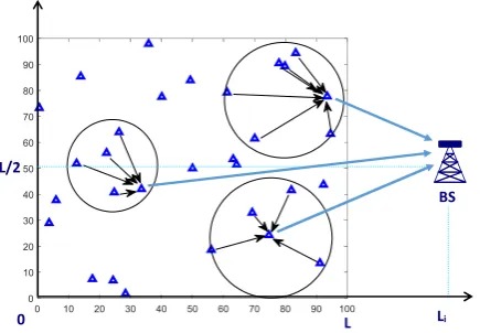
5. Cluster-Based Data Collection

5.1. Network Model

In this section, we assume to haveN sensors randomly distributed in a sensing area. We consider both circular and square shapes of the are need to be observed. We assume that a certain number of nodes (Nc) are

randomly chosen as cluster-heads (CH). The other nodes choose the closest CH to join the cluster. We use K-means [20] and LEACH [21] in simulation to compare to our analysis results later. We consider the data collection ideas from [36, 37]. In [36], all sensor

10003 1100 1200 1300 1400 1500 1600 1700 1800 1900 2000 3.5

4 4.5 5 5.5 6 6.5x 10

5

Number of sensors in the networks

T

o

ta

l

p

o

w

e

r

c

o

n

s

u

m

p

ti

o

n

Total power consumption in arbitrary networks

Analysis Simulation

Figure 8. Total power consumption in random networks with different number of sensors, transmission range R = 8 when the BS at the center of the sensing area

readings from each cluster are added up together and there are only a certain number of measurements are sent to the BS directly, denoted as DCCS. In [37] the measurements are forwarded in multi-hop routing between intermediate CHs to the BS, denoted as ICCS.

5.2. Communication Power Consumption Analysis

We define the power consumption associated with all data transmission between non-CH nodes and the CHs that they belong to as intra-cluster power consumption, denoted as Pintra−cluster. The CHs can create a certain

number of measurements as combinations of all received data within each cluster and finally send the CS measurements directly or in multi-hop to the BS. The corresponding power consumption is referred to as

Pto BS. The total power consumption for all transmission

in such network is calculated as

Ptotal = (Pintra−_cluster+P_{to BS}). (27)

We consider both sensing areas, square dimensioned L×_{L Land circular with radiusR0. In each area, both}

methods DCCS and ICCS are formulated.

Working on a square sensing area. In order to analyze the network, we assume to have an uniformly distributed WSN divided intoNcclusters with the same number of

sensors asN /Nc, consisting of only one CH and (NNc

−₁₎

non-CH sensors. We achieve

Pintra−cluster =NC(N Nc

−_1)E[rα_{], (28)}

calculateE[r2] as follows.

E[r2] =

Z Z

(x2+y2)ρ(x, y)dx dy (29)

=

Z Z

r02ρ(r0, θ)r0dr0dθ, (30)

whereρ(x, y) is called a node distribution. We assume each cluster area is a circle with radius R=L/√πNc

and the density of the nodes is uniform throughout the cluster area, i.e.ρ(r0, θ) = 1/(L2/Nc). Finally we obtain

E[r2] = 1 (L2_/N

c)

Z 2π

θ=0

Z R

r0

=0

r03dr0dθ= L

2

2πNc

, (31)

and accordingly

Pintra−cluster = (N Nc

−₁₎L 2

2π. (32)

As we see, the total intra-cluster power consumption is a decreasing function of the number of clusters.

*Analysis ofPto BS to forward directly the

measure-ments to the BS (DCCS):

We assume the BS is located at the location (Li,L2)

with respect to our reference point (see Figure 9). The

0 10 20 30 40 50 60 70 80 90 100 0

10 20 30 40 50 60 70 80 90 100

0 L

L/2

Li

BS

Figure 9. A WSN has more than three clusters with the BS outside the sensing area (Li > L).

average consumed power by all CHs is given by

Pto BS =ME[d2], (33)

where d is considered to be a random variable that represents a distance between a CH and the BS. It is assumed that all CHs are randomly distributed in the sensing area. The expected squared distance between all CHs and the BS is calculated in Equation13

in Section 3.2. We finally obtain the total power consumption for the network as

Ptotal = ( N Nc

−₁₎L 2

2π+ M

L [

(L−_Li)3_+L3

i

3 ] +

ML2

12 (34)

We usually have two common positions for the BS, at the center of the sensing area (Li =L/2) and outside

the sensing area (Li ≥L). For the former case, (34) is

simplified as

Ptotal = ( N Nc

−₁₎L 2

2π + ML2

6 . (35)

Working on a circular sensing area. We assume to have a uniformly distributed WSN divided intoNc clusters

with the same number of sensors asN /Nc, consisting of

one CH and (_NN

c−1) non-CH nodes. We first calculate

the intra-cluster power consumption as

Pintra−_cluster=N_c( N Nc

−_1)E[r2_{], (36)}

Similar to Equation30, we can calculateE[r2] as follows

E[r2] =

Z Z

r02ρ(r0, θ)r0dr0dθ, (37)

where ρ(r0, θ) is the node distribution as ρ(r0, θ) = 1/(πR2₀/Nc). We assume each cluster area is a circle with

radiusRc=R0/ √

Nc. Equation37is rewritten as

E[r2] = 1 (πR2₀/Nc)

Z 2π

θ=0

Z R_c

r0

=0

r03dr0dθ= R

2 0

2Nc

, (38)

and accordingly

Pintra−_cluster= ( N Nc

−₁₎R 2 0

2 . (39)

We can also see that the total intra-cluster consumed power is a decreasing function of the number of clusters.

Next, we need to find the power consumption to forward M measurements to the BS, Pto BS, which is

based on the distances between CHs and the BS. As mentioned, there are two methods, DCCS and ICCS which are addressed as follows.

*Analysis ofPto BS to forward directlyM

measure-ments to the BS (DCCS):

The mean value of consumed power to transmit data from any random CH to the BSE[d_toBS2 ] can be calcu-lated following the same idea mentioned in [11], while dtoBS represents a real transmitting distance from any

CH to the BS, as shown in Figure10.

Since sensors are uniformly randomly distributed in the model and the CHs are also chosen randomly, we can say thatdtoBS can be consider as a random variable

(r). And the maximum distance is the radius of the circle areaR0. The mean value of the square distance can be

calculated as follows

E[d_toBS2 ] =

Z Z

(x2+y2)ρ(x, y)dx dy (40)

=

Z Z

0 20 40 60 80 100 0

10 20 30 40 50 60 70 80 90 100

N=2000 random sensors distributed in a circle

Figure 10. Consider real distances from CHs to the BS in a circular area arbitrary network

Assumed all sensors or CHs are uniformly distributed in the circular area with the radius R0, and ρ(x, y) =

1/(πR2₀) is the uniform distribution of CHs (pdf), and BS is at the center of the sensing area. We obtain the average power consumption for each measurement transmitted from a random CH to the BS as

E[d_toBS2 ] = 1 πR2₀

Z2π

θ=0

ZR₀

r=0

r3dr dθ (42)

=R

2 0

2 . (43)

Finally, we have the total power consumption for such networks

Ptotal = (N Nc

−₁₎R 2 0

2 +M

R2₀

2 . (44)

* Analysis of PtoBS to forward M measurements

through inter-cluster multi-hop (ICCS):

In case we apply inter-cluster multi-hop relaying data through CHs, we need the average number of hops from Equation22to calculate the total power consumption as

Ptotal = ( N Nc

−₁₎R 2 0

2 +PtoBS, (45)

wherePtoBScan be calculated as

PtoBS =M       

N oHmax−

N oHmax−1 X

n=1

Pn(x) PN oH_max(x)

      

Rαc, (46)

andRcis the transmission range for each CH to create

a tree for routing data. The tree can be formed as tree-based routing, mentioned in the previous section.

5.3. Simulation Results

In this section we consider circular sensing area with radius R0= 50. There are 2000 sensor nodes are

deployed randomly the sensing area. The network is divided into different number of clusters of Nc=

[100, 200, 300, 400] that corresponds to the CH’s transmission rangeRc= [25, 22, 18, 14].

100 150 200 250 300 350 400

Different number of clusters

0.5 1 1.5 2 2.5 3 3.5 4

T

o

ta

l

in

tra

-c

lu

s

te

r

p

o

w

e

r

c

o

n

s

u

m

p

tio

n

104 _{Compare total intra-cluster power consumption}

Analysis K-means

Figure 11. Total intra-cluster power consumption when N =

2000 sensors deployed in a circular sensing area withR0= 50;

BS at the center

Figure 11 depicts the total intra-cluster power con-sumption (Pintra−_cluster) as formulated in Equation 39. The analysis result is also compared with another net-work clustered by K-means. In our formula we assume to have all clusters with equal size. So, in the figure, both the power consumption values at different number of clusters are quite similar.

0 50 100 150 200 250 300 350 400

Different number of clusters 3

4 5 6 7 8 9 10 11 12 13

In

te

r-c

lu

s

te

r

P

o

w

e

r

C

o

n

s

u

m

p

ti

o

n

105 _{Inter-clusters multihop routing(Nc = 10 -> 400)}

Analysis K-means

Figure 12. An illustration of a total inter-cluster power consumption; a WSN with 2000 sensors randomly deploying in a

circular sensing area (R0= 50; BS at the center)

the BS in multi-hop through intermediate CHs, as formulated in Equation 46. Our analysis result is also compared with an arbitrary network clustered by K-means clustering algorithm. All the equations are classified well when both analysis and simulation results come very close to each other.

6. Neighborhood-Based Data Collection

6.1. Network Model

We assume to haveN sensors are randomly distributed in a sensing area. Given an appropriate transmission rangeR, all the sensors are connected as an undirected graph G(V, E), whereV is the set of vertexes is always equal toN.Eis the set of edges that counts the possible communication links between the sensors depending on the value of transmission range R. As mentioned in [26],Mrandom sensors out ofN are chosen to collect sensor readings from their own neighbors’ including themselves to create CS measurements. After that, these M measurements are sent to the BS directly or are relayed through intermediate nodes.

6.2. Communication Power Consumption Analysis

The total power consumption for all data transmissions as mentioned in the network model has two main parts, the power consumed for transmission between M neighborhoods denoted asPnei and the other one to

forwardM measurements to the BS, denoted as Pto BS,

as shown as bellows

Ptotal= (Pnei+Pto BS). (47)

We assume that each neighborhood has the same number of sensors that depends on the sensor density of the network.Pneiis calculated as

Pnei=ω×R2×M, (48)

where ω represents an average number of neighbors that each sensor can have. It is assumed that sensors are randomly distributed in the area. The average number of nodes can be calculated depending on the area covered by each sensor transmission rangeRas N

R2₀×R

2_.

By analyzed, we can calculate the mean value asω as follows.

ω= (NR

2

R2₀

−_{1). (49)}

Hence, the total consumed power for data gathering in Mneighborhoods is calculated as

Pnei= (N R2 R2₀

−_1)R2_{M. (50)}

* Note that in a square sensing area,ωis calculated differently as

ω= (NπR

2

L2 −1). (51)

* Analysis of Pto BS to forward directly M

measure-ments to the BS (DirectNei)

Each chosen node after generating the measurement transmits directly it to the BS. We can calculate Pto BS

based on Equation43and finally obtain the total power consumption in this case as

Ptotal = (N R2 R2₀

−_1)R2_M+R 2 0

2 M. (52)

* Analysis ofPto BS to forward M measurements in

multi-hop to the BS (Multi-hopNei)

In other case we choose to transmit data from each neighborhood to the BS through intermediate nodes by multi-hop routing, Pto BS can be calculated based on

Equation 22 to calculate the average number of hops from each neighborhood to the BS. Finally, the total power consumption in this case is

Ptotal= (N R2

R2₀

−_1)R2_{M+Pto BS, (53)}

wherePto BSis

Pto BS =M

      

N oHmax−

N oHmax−1 X

n=1

Pn(x) PN oH_max(x)

      

R2. (54)

6.3. Simulation Results

In this section, we consider a circular sensing area and deploy different number of sensors randomly on it. We chose a fixed a sensor transmission range R= 9 and guaranteed that the network is always connected. Our goal is to verify our formulas in arbitrary networks.

Figure 13 depicts the total intra-neighborhood power consumption from all N sensor nodes. As we increase the number of nodes, this power consumption increases. The gap between our analysis and simulation results also increases. In analysis case, we assumed that all sensors have the same number of neighbors but in an arbitrary network, sensors close to the boundary have less neighbors than the ones in the middle of the sensing area. We can increase the transmission range to reduce the error of calculation between these two results.

We consider that each sensor uses tree-based routing tree [26] to relay the data to the BS at the center of the sensing area. Figure 14depicts the total power for all the sensors (different numbers of sensors are deployed) send their data to the BS through the intermediate nodes to the BS.

In Figure15 we calculate the total power consump-tion based on Equaconsump-tions (52) and (53) for both ways to transmit a certain number (M) of measurements to the BS. If we do not consider network latency or capacity, transmitting in multi-hop (Multi-hopNei) con-sumes 30−_{40% less power than transmitting directly}

500 600 700 800 900 1000 1100 1200 1300 1400 1500 0

1 2 3 4 5

6x 10

6 Total intra-neighborhood power consumption (P_nei)

Number of nodes in the network (number of neighborhoods)

A

v

e

ra

g

e

t

o

ta

l

p

o

w

e

r

c

o

n

s

u

m

p

ti

o

n

Analysis Simulation

Figure 13. Total intra-neighborhood power consumption with different number of sensors deployed in a circular sensing area

600 700 800 900 1000 1100 1200 1300 1400 1500 1600

0.5 1 1.5 2 2.5 3 3.5 4 4.5

5x 10

6 _{Total power consumption arbitrary networks ( cicular area )}

Number of sensors deployed in the networks

A

v

e

ra

g

e

t

o

ta

l

p

o

w

e

r

c

o

n

s

u

m

p

ti

o

n

Analysis Simulation

Figure 14. Total power consumption with different number of sensors deployed in a circular sensing area; multi-hop routing is applied to transmit data from each neighborhood to the BS at the center of the sensing area

90 95 100 105 110 115 120 125 130 135 140

1 1.5 2 2.5 3 3.5x 10

5 _{Total power consumption (N = 500, R = 9)}

Number of measurements

A

v

e

ra

g

e

t

o

ta

l

p

o

w

e

r

c

o

n

s

u

m

p

ti

o

n

DirectNei Analysis DirectNei Simulation Multi-hopNei Analysis Multi-hopNei Simulation

Figure 15. Total power consumption with different number of measurements sending to the base-station (BS) in both methods are compared; The BS is at the center of the sensing area; N =

500 sensors; transmission rangeR= 9

7. Conclusions

In this paper, we formulate the average power con-sumptions for data transmission in WSNs based on stochastic problems. Almost the common net-work topologies such as tree-based, random walk, neighborhood-based and cluster-based are considered. The consumed powers of power amplifiers at sensors which are function of transmitting distances are formu-lated as average power consumptions. All transmitting power consumptions are formulated for such network topologies. Both analysis and simulation results are addressed to compare and verify the formulas. Based on the results, some optimal cases are suggested for such networks to minimize power consumption in order to prolong the network lifetime.

In future work, we focus on different distributions of sensors deploying in sensing areas to calculate power consumption. Some general calculations could be provided for hybrid networks. Based on those ideas, either WSNs or MSNs can be managed better with longer time of operation.

Acknowledgement

This work was supported in part by the Newton Fund Institutional Link through the Fly-by Flood Monitoring Project under Grant ID 428328486, which is delivered by the British Council.

References

[1] D. Puccinelli and M. Haenggi, “Wireless sensor net-works: applications and challenges of ubiquitous sens-ing,”Circuits and Systems Magazine, IEEE, vol. 5, no. 3, pp. 19–31, 2005.

[2] M. T. Nguyen, Data Collection Algorithms in Wireless

Sensor Networks Employing Compressive Sensing. PhD

thesis, Oklahoma State University, 2015.

[3] J. Al-Karaki and A. Kamal, “Routing techniques in wire-less sensor networks: a survey,”Wireless Communications, IEEE, vol. 11, pp. 6–28, Dec 2004.

[4] P. Gupta and P. R. Kumar, “Critical power for asymptotic connectivity in wireless networks,” pp. 547–566, 1998. [5] F. Xue and P. R. Kumar, “The number of neighbors

needed for connectivity of wireless networks,” Wirel. Netw., vol. 10, pp. 169–181, Mar. 2004.

[6] Q. Wang, M. Hempstead, and W. Yang, “A realistic power consumption model for wireless sensor network devices,” in3rd Annual IEEE Communications Society on Sensor and Ad Hoc Communications and Networks, vol. 1, pp. 286–295, Sept 2006.

[7] H. Q. Ngo, L. Tran, T. Q. Duong, M. Matthaiou, and E. G. Larsson, “On the total energy efficiency of cell-free massive mimo,” IEEE Transactions on Green

Communications and Networking, vol. 2, pp. 25–39,

March 2018.

management for small-cell heterogeneous networks with limited backhaul capacity,”IEEE Transactions on Wireless Communications, vol. 16, pp. 872–884, Feb 2017. [9] L. Lovász, “Random walks on graphs: A survey,” 1993. [10] M. Nguyen and Q. Cheng, “Efficient data routing

for fusion in wireless sensor networks,” in The 25th International Conference on Computer Applications in Industry and Engineering (CAINE), New Orleans, LA, Nov 2012.

[11] M. T. Nguyen, “Minimizing energy consumption in random walk routing for wireless sensor networks utilizing compressed sensing,” in System of Systems Engineering (SoSE), 2013 8th International Conference on, pp. 297–301, June 2013.

[12] H. Tian, H. Shen, and T. Matsuzawa, “Randomwalk routing for wireless sensor networks,” in Parallel and Distributed Computing, Applications and Technologies,

2005. PDCAT 2005. Sixth International Conference on,

pp. 196–200, Dec 2005.

[13] C. M. Angelopoulos, S. Nikoletseas, D. Patroump, and C. Rapropoulos, “A new random walk for efficient data collection in sensor networks,” inProceedings of the 9th ACM International Symposium on Mobility Management and Wireless Access, MobiWac ’11, (New York, NY, USA), pp. 53–60, ACM, 2011.

[14] L. Lima and J. Barros, “Random walks on sensor networks,” in Modeling and Optimization in Mobile, Ad Hoc and Wireless Networks and Workshops (WiOpt 2007). 5th International Symposium on, pp. 1–5, April 2007. [15] S. Boyd, P. Diaconis, and L. Xiao, “Fastest mixing markov

chain on a graph,”SIAM REVIEW, vol. 46, pp. 667–689, 2003.

[16] R. Bellman, “On a routing problem,”Quart. Appl. Math., vol. 16, pp. 87–90, 1958.

[17] J. M. Steele, “Minimal spanning trees for graphs with random edge lengths,” in Mathematics and computer science, II (Versailles, 2002), Trends Math., pp. 223–245, Basel: Birkhäuser, 2002.

[18] R. Xie and X. Jia, “Minimum transmission data gathering trees for compressive sensing in wireless sensor networks,” in Global Telecommunications Conference

(GLOBECOM 2011), 2011 IEEE, pp. 1–5, 2011.

[19] M. T. Nguyen and K. A. Teague, “Tree-based energy-efficient data gathering in wireless sensor networks deploying compressive sensing,” in 23rd Wireless and Optical Communication Conference (WOCC), pp. 1–6, May 2014.

[20] J. B. MacQueen, “Some methods for classification and analysis of multivariate observations,” in Proc. of the fifth Berkeley Symposium on Mathematical Statistics and Probability(L. M. L. Cam and J. Neyman, eds.), vol. 1, pp. 281–297, University of California Press, 1967. [21] W. Heinzelman, A. Chandrakasan, and H. Balakrishnan,

“An application-specific protocol architecture for wire-less microsensor networks,” Wireless Communications, IEEE Transactions on, vol. 1, pp. 660 – 670, Oct 2002. [22] M. Handy, M. Haase, and D. Timmermann, “Low energy

adaptive clustering hierarchy with deterministic cluster-head selection,” in 4th Int. Workshop on Mobile and Wireless Communications Network, pp. 368–372, 2002. [23] G. Gupta and M. Younis, “Load-balanced clustering of

wireless sensor networks,” inCommunications, 2003. ICC

’03. IEEE International Conference on, vol. 3, pp. 1848 – 1852 vol.3, May 2003.

[24] S. Bandyopadhyay and E. Coyle, “An energy efficient hierarchical clustering algorithm for wireless sensor net-works,” inINFOCOM 2003. Twenty-Second Annual Joint Conference of the IEEE Computer and Communications.

IEEE Societies, vol. 3, pp. 1713–1723 vol.3, Mar-Apr

2003.

[25] O. Younis and S. Fahmy, “Distributed clustering in ad-hoc sensor networks: a hybrid, energy-efficient approach,” inINFOCOM 2004. Twenty-third AnnualJoint Conference of the IEEE Computer and Communications Societies, vol. 1, pp. 4 vol. (xxxv+2866), Mar 2004. [26] M. T. Nguyen and K. A. Teague, “Neighborhood based

data collection in WSNs employing compressive sens-ing,” in The International Conference on Advanced Tech-nologies for Communications (ATC’14), (Hanoi, Vietnam), Oct. 2014.

[27] M. T. Nguyen and K. A. Teague, “Compressive and cooperative sensing in distributed mobile sensor networks,” in MILCOM 2015 - 2015 IEEE Military Communications Conference, pp. 1033–1038, Oct 2015. [28] M. T. Nguyen and K. A. Teague, “Random sampling

in collaborative and distributed mobile sensor networks utilizing compressive sensing for scalar field mapping,”

in 2015 10th System of Systems Engineering Conference

(SoSE), pp. 1–6, May 2015.

[29] H. M. La and W. Sheng, “Dynamic target tracking and observing in a mobile sensor network,” Robotics and Autonomous Systems, vol. 60, no. 7, pp. 996 – 1009, 2012. [30] H. La, W. Sheng, and J. Chen, “Cooperative and active sensing in mobile sensor networks for scalar field mapping,” 2014.

[31] D.L.Donoho, “Compressed sensing,”Information Theory, IEEE Transactions on, vol. 52, pp. 1289 – 1306, 2006. [32] E. Candes, J. Romberg, and T. Tao, “Robust uncertainty

principles: exact signal reconstruction from highly incomplete frequency information,”Information Theory, IEEE Transactions on, vol. 52, pp. 489 – 509, Feb. 2006. [33] T. S. Rappaport,Wireless Communications: Principles and

Practice (2nd Edition). Prentice Hall, 2 ed., Jan. 2002. [34] S. Chandler, “Calculation of number of relay hops

required in randomly located radio network,”Electronics Letters, vol. 25, no. 24, pp. 1669–1671, 1989.

[35] M. T. Nguyen and K. A. Teague, “Neighborhood based data collection in WSNs employing compressive sens-ing,” in The International Conference on Advanced Tech-nologies for Communications (ATC’14), (Hanoi, Vietnam), Oct. 2014.

[36] M. T. Nguyen and N. Rahnavard, “Cluster-based energy-efficient data collection in wireless sensor networks utilizing compressive sensing,” in Military

Communications Conference, MILCOM 2013 - 2013 IEEE,

pp. 1708–1713, Nov 2013.