R E S E A R C H
Open Access
A customized proximal point algorithm
for stable principal component pursuit with
nonnegative constraint
Kaizhan Huai
*, Mingfang Ni, Feng Ma and Zhanke Yu
*Correspondence:
[email protected] College of Communications Engineering, PLA University of Science and Technology, Nanjing, 210007, China
Abstract
The stable principal component pursuit (SPCP) problem represents a large class of mathematical models appearing in sparse optimization-related applications such as image restoration, web data ranking. In this paper, we focus on designing a new primal-dual algorithm for the SPCP problem with nonnegative constraint. Our method is based on the framework of proximal point algorithm. By taking full exploitation to the special structure of the SPCP problem, the method enjoys the advantage of being easily implementable. Global convergence result is established for the proposed method. Preliminary numerical results demonstrate that the method is efficient.
Keywords: proximal point method; customized; stable principal component pursuit; primal-dual algorithm
1 Introduction
With the development of information technology, the subject of high-dimensional data becomes more and more popular in science and engineering applications such as image and video processing, web documents analysis and bioinformatics data processing. An in-tensive research attention has been devoted recently to analyzing, processing and exacting useful information from the high-dimensional data efficiently and accurately. The classi-cal principal component analysis (PCA) is the most widely used tool for high-dimensional data analysis, and it plays a fundamental role in dimensionality reduction. PCA computes the singular value decomposition (SVD) of a matrix to obtain a low-dimensional approx-imation to high-dimensional data in thesense []. However, PCA usually breaks down when the given data is corrupted by gross errors. In other words, the classical PCA is not robust to gross errors or outliers. To overcome this issue, many methods have been pro-posed. In [], a new model called principal component pursuit (PCP) was proposed by Candès and Wright under weak assumptions. It is assumed that the matrixM∈Rm×nis
of the formM=L+S, whereLis the underlying low-rank matrix representing the prin-ciple components andSis a sparse matrix with its most entries being zero. To recoverL
andS, PCP requires to solve the following convex optimization problem:
min L∗+ρS
s.t.L+S=M,
L,S∈Rm×n,
(.)
whereL∗ denotes the nuclear norm ofL, which is equal to the sum of its singular val-ues,S=i,j|Si,j|is thenorm ofS, andρis a parameter balancing the low-rank and sparsity.
In [], it was shown that the recovery is still feasible even when the data matrixMis cor-rupted with a dense error matrixZsuch thatZF≤δ. Indeed, this can be accomplished
by solving the following stable principal component pursuit (SPCP) problem:
min L∗+ρS
s.t.L+S+Z=M,
ZF≤σ,
L,S,Z∈Rm×n,
(.)
where the matrixZis the noise,ZF denotes the Frobenius norm ofZ, andσ> is the
noise level. Note that (.) is a special case of the SPCP problem (.) withσ= . In practi-cal applications such as background exacting from face recognition, video denoising and surveillance video, the low-rank matrixLalways represents an image. Therefore, adding a nonnegative constraintL≥ to (.) makes sense. This results in the following SPCP problem with nonnegative constraint:
min L∗+ρS+I(ZF≤σ) +I(L≥)
s.t.L+S+Z=M,
L,S,Z∈Rm×n,
(.)
whereI(·) is an indicator function [].
The rest of this paper is organized as follows. In Section , we give some useful prelimi-naries. In Section , we present the customized PPA for solving (.) and the convergence analysis is shown in Section . In Section , we compare our algorithm with APGM to illustrate the efficiency by performing numerical experiments. Finally, some conclusions are drawn in Section .
2 Preliminaries
In order to facilitate the analysis, we consider the following separable convex optimization problem with linear constraint instead of (.):
min f(x) +g(y)
s.t.Ax+By=b,
x∈X, y∈Y,
(.)
whereA∈Rm×n,B∈Rm×p,b∈Rm,X⊆RnandY⊆Rpare convex sets, andf(x) :Rn→ Randg(y) :Rp→Rare both convex but not necessarily smooth functions [].
Through-out, the solution set of (.) is assumed to be nonempty. Furthermore, we assume that f(x) andg(y) are ‘simple’ which means that their proximal operators have a closed-form representation or they can be efficiently solved up to a high precision []. The proximal operator of the functionϕ(x) :Rn→Ris defined as
Prox(ϕ,ξ,a) =argmin
ϕ(x) + ξx–a
x∈X
(.)
for any givena∈Rnandξ> []. The nuclear norm ofLand the
norm ofSin (.) both are simple functions. Under the assumption, we will show that our algorithm for solving (.) can result in easy proximal subproblems.
We signify the subdifferential of the convex functionf(x) by∂f(x),
∂f(x) :=d∈Rn|f(z) –f(x)≥dT(z–x),∀z∈Rn, (.) and eachd∈∂f(x) is called a subgradient off(x) []. Letθ(x)∈∂f(x), then we can have
f(z) –f(x)≥(z–x)Tθ(x), (.a)
f(x) –f(z)≥(x–z)Tθ(z). (.b)
Merging (.a) and (.b), we can easily get
(x–z)Tθ(x) –θ(z) ≥, ∀x,z∈Rn, (.)
which implies that the mappingθ(·) is monotone.
Now, we show that (.) can be characterized by a variational inequality (VI) framework. Letλ∈Rmbe the Lagrangian multiplier associated with the linear constraint in (.), then the Lagrangian function of (.) is
By deriving the optimality conditions of (.), we can easily find that solving (.) is equiv-alent to finding a pair of (x∗,y∗;λ∗) which satisfies
⎧ ⎪ ⎨ ⎪ ⎩
x∗∈X, (x–x∗)T(θ(x∗) –ATλ∗)≥, ∀x∈X,
y∗∈Y, (y–y∗)T(γ(y∗) –BTλ∗)≥, ∀y∈Y,
Ax∗+By∗–b= ,
(.)
whereθ(x∗)∈∂f(x∗) andγ(y∗)∈∂g(y∗). By denoting
u=
x y
, w=
⎛ ⎜ ⎝ x y λ ⎞ ⎟
⎠, h(u) =f(x) +g(y), F(w) = ⎛ ⎜ ⎝
–ATλ
–BTλ
Ax+By–b ⎞ ⎟
⎠, (.a)
and
=X×Y×Rm, (.b)
problem (.) can be rewritten as the variational inequality reformulation
w∗∈, h(u) –hu∗ +w–w∗ TFw∗ ≥, ∀w∈. (.)
Obviously, the mappingF(w) defined in (.a) is monotone. The solution set of (.a)-(.), denoted by∗is nonempty under the assumption that the solution set of (.) is not empty.
3 The new algorithm
In this section, we will present our new algorithm to solve VI (.). However, at the begin-ning, we first review the classical PPA.
After the PPA was proposed firstly by Martinet in [] and further developed by Rock-afellar in [], it plays a vital role in optimization area. Given the iteratewk, the classical
PPA generates the new iteratewk+∈via the following procedure:
h(u) –huk+ +w–wk+ TFwk+ +Gwk+–wk ≥, ∀u∈, (.)
where the metric proximal parameterG∈Rn×nis required to be a positive definite matrix.
A popular choice ofGisG=βI, whereβ> andIis the identity matrix []. Here, we are ready to present our new algorithm for solving (.).
Algorithm (The main algorithm for (.))
Letr> ands>rBTB, take(x,y;λ)∈X×Y×Rmas the initial point. Step . Updatey,xandλ:
yk+=argmin
g(y) +r
y–yk– rB
Tλk
y∈Y
,
xk+=argmin
f(x) –
λk– s
Axk+Byk+–yk –b
T
+ sA
x–xk + x–x
k x∈X
,
λk+=λk– s
Axk++Byk+–yk –b .
Step . If the termination criterion is met, stop the algorithm; otherwise, go to Step .
The new customized PPA described above is known as alternating direction method of multipliers (ADMM) with two blocks []. Its global convergence result has been proven in many literature works. However, there are three variables in (.). If we apply the cus-tomized PPA to the SPCP problem directly, the convergence of the algorithm cannot be guaranteed []. Moreover, the proximal mapping ofL∗+I(L≥) is difficult to com-pute []. By introducing a new auxiliary parameterK, we can groupLandSas one big block [L;S], and groupZandKas another big block [Z;K]. Then (.) can be rewritten as a similar form of (.):
minL,S,Z,KL∗+ρS+I(ZF≤σ) +I(K≥)
s.t. I I Z K + I I –I L S = M . (.)
Then we can solve (.) or (.) by applying the new customized PPA as follows:
Lk+=argminL∗+r
L–Lk– r
k–k
F
, (.a)
Sk+=argminρS+r
S–Sk– r k F , (.b)
Zk+=argminIZF≤σ
+ +s s
Z–Zk– +s
sk–Lk+–Lk+ Sk+–Sk+Zk–M
F
, (.c)
Kk+=argminI(K≥) + +s
s
K–Kk– +s
sk–Lk– Lk++Kk+M
F
, (.d)
k+=k– s
Lk+–Lk+ Sk+–Sk+Zk+–M , (.e) k+=k–
s
Kk++Lk– Lk+ . (.f)
The simplicity of the above scheme is that all the subproblems have closed-form solutions. As we see, model (.) turns out to be (.) when we setσ> and abandon the constraint L≥. Under these circumstances, subproblems (.a) and (.b) are the solution of (.). We now show the reason that the four subproblems can be solved easily. The first sub-problem (.a) is equivalent to solving the proximal mapping of the nuclear normL∗
and can be expressed by
Lk+:=MatShrink
Lk+ r
k–k , r
where the matrix shrinkage operationMatShrink(M,α) (α> ) is defined as
MatShrink(M,α) :=UDiagmax{σ–α, } VT,
andUDiag(σ)VTis the SVD of the matrixM, see [] and [].
TheS-subproblem (.b) can be solved by
Sk+:=Shrink
Sk+
r
k
, ρ r
, (.)
where theshrinkage operator []Shrink(M,α) is defined as
Shrink(M,α)ij:= ⎧ ⎪ ⎨ ⎪ ⎩
Mij+α, ifMij< –α,
Mij–α, ifMij>α,
, if|Mij| ≤α.
The closed-form solution of the third subproblem (.c) can be written as
Zk+:=Wk/max,WkF/σ, (.)
which means projecting the matrixWk:=M+sk
– (Lk+–Lk+ Sk+–Sk) onto the Euclidean ballZF≤σ. TheK-subproblem (.d) corresponds to projecting the matrix
(Lk+–Lk+sk
–M) onto the nonnegative orthant and this can be done by
Kk+:=maxLk+–Lk+sk–M, , (.)
where the max function is componentwise [].
4 Convergence analysis
In this section, we will show the global convergence result of the algorithm proposed for solving (.) or (.). First, we need to prove the following lemma.
Lemma Let wk+= (xk+,yk+;λk+)be generated by the proposed algorithm from the given wk= (xk,yk;λk).Then we can have
h(u) –huk+ +w–wk+ TFwk+ +Gwk+–wk ≥, ∀w∈, (.)
where
G= ⎛ ⎜ ⎝
I rI BT
B sI
⎞ ⎟ ⎠.
Proof Deriving the first-order optimality condition of the first equality in Algorithm , we can obtain
It can also be expressed as
g(y) –gyk+ +y–yk+ TBTλk+–λk –BTλk++ryk+–yk ≥, ∀y∈Y. (.) Homoplastically, the second iteration for solvingxk+in Algorithm shows us that
f(x) –fxk+ +x–xk+ T
–Aλk+ sA
TAxk+Byk+–yk –b
+
I+ sA
TAxk+–xk ≥, ∀x∈X. (.)
Substitutingλk=λk++
s(Axk++B(yk+–yk) –b) into (.), we get
f(x) –fxk+ +x–xk+ T–ATλk++xk+–xk ≥, ∀x∈X. (.)
Note that theλ-iteration can be written as
Axk++Byk+–b+Byk+–yk +sλk+–λk = . (.) Merging (.), (.) and (.), we achieve
h(u) –huk+ + ⎛ ⎜ ⎝
x–xk+ y–yk+ λ–λk+
⎞ ⎟ ⎠
T
× ⎧ ⎪ ⎨ ⎪ ⎩ ⎛ ⎜ ⎝
–ATλk+ –BTλk+ Axk++Byk+–b
⎞ ⎟ ⎠+
⎛ ⎜ ⎝
(xk+–xk)
r(yk+–yk) +BT(λk+–λk)
B(yk+–yk) +s(λk+–λk)
⎞ ⎟ ⎠ ⎫ ⎪ ⎬ ⎪
⎭≥, ∀w∈. (.)
Utilizing the notation ofw,F(w) and the matrixG, the inequality above can be rewritten as
h(u) –huk+ +w–wk+ TFwk+ +Gwk+–wk ≥, ∀w∈. (.) In other words, the lemma is proved. Inequality (.) implies that the proposed algorithm is in fact equivalent to the proximal point algorithm with a special proximal regularization
parameter matrixG.
Now we show and prove the contractive property of the proposed algorithm.
Lemma Assume that the parameters r> and s>rBTBare satisfied.Let wk+be the sequence generated by the new algorithm with an arbitrary initial iterate w.Then it holds
wk+–w∗G ≤wk–w∗G –wk+–wkG, ∀w∗∈∗. (.)
The norm · Gis defined aswG=w,Gwand the corresponding inner product·,·Gis
Proof Becausew∗∈∗ is optimal to (.), it follows from the KKT conditions that the following hold:
∈∂fx∗ –ATλ∗, (.a)
∈∂gy∗ –BTλ∗, (.b)
=Ax∗+By∗–b. (.c)
As we see, the optimality condition for the first subproblem in Algorithm is
∈∂gyk+ +r
yk+–yk– rB
Tλk
. (.)
Combining (.b) and (.) under the fact thatθ(·) is monotone, we have
yk+–y∗ TBTλk–ryk+–yk –BTλ∗ ≥. (.)
Similarly, the optimality condition for the subproblem with respect toxcan be given by
∈∂fxk+ –AT
λk– s
Axk++Byk+–yk –b
+ sA
TAxk+–xk +xk+–xk . (.)
Substituting theλ-subproblem into (.), we obtain
∈∂fxk+ –ATλk++xk+–xk . (.)
Combining (.a) and (.), we get
xk+–x∗ TATλk+–xk+–xk –ATx∗ ≥. (.)
Summing (.) and (.), we can achieve
xk+–x∗ TATλk+–λ∗ +xk+–x∗ Txk–xk+ +yk+–y∗ TBTλk–λk+ +yk+–y∗ TBTλk+–λ∗ +ryk+–y∗ Tyk–yk+ ≥. (.)
Combining theλ-subproblem with (.c), we get
λk+–λ∗ TByk+y∗– yk+ –Axk+–x∗ +sλk–λk+ ≥. (.)
Note that (.) can be rewritten as
λk+–λ∗ TByk–yk+ +sλk+–λ∗ Tλk–λk+
Using the definition of·,·Gand (.), we have
wk+–w∗,wk–wk+!G
≥xk+–x∗ TATλk+–λ∗ +xk+–x∗ Txk–xk+ +yk+–y∗ TBTλk–λk+ +ryk+–y∗ Tyk–yk+
+yk+–y∗ TBTλk+–λ∗ . (.)
Recall (.), we can easily get
wk+–w∗,wk–wk+!G≥. (.)
Therefore
wk+–wk,w∗–wk!G≥wk+–wkG. (.)
Combining (.) with the identity
wk+–w∗G=wk+–wkG– wk+–wk,w∗–wk!G+wk–w∗G, (.)
we get
wk+–w∗G≤wk–w∗G–wk+–wkG. (.)
This completes the proof. Note that the sequence{wk}is Fejér monotone with respect to the solution set. In addition, the proposed algorithm to solve (.) or (.) has the frame-work of contraction type methods. Therefore, by using the Fejér monotonicity and the contractility, the rest of the convergence proof becomes standard. Here, we do not repeat.
We refer the readers [] for more details.
5 Numerical results
In this section, we study the performance of Algorithm for solving (.). Our codes were written in MATLAB Ra. In addition, all of the experiments were performed on a lap-top with an Intel Core Duo CPU at . GHz and GB memory. In the experiments, we get the data randomly in the same way as in []. For givenn,r<n, then×nmatrixL∗with rank-rwas generated byRRT, whereRandRare both random matrices with all compo-nents distributed in [, ] uniformly. As we see,L∗is a nonnegative and low-rank matrix we want to recover. The support of the sparse matrixS∗was chosen uniformly at random, and the nonzero components ofS∗were drawn uniformly in the interval [–, ]. The components of matrixZ∗for noise were generated as i.i.d. Gaussian with standard devi-ation –. Then we setM=L∗+S∗+Z∗. According to the suggestion in [], we chose ρ= /√n. The starting point for the two algorithms was set asL=K= –M,S=Z= , == . In our experiments, we use
resid = L+S+Z–MF MF
Table 1 Comparison of the CPU times between APGM and Algorithm 1
n Algorithm Rr= 0.01,Cr= 0.01 Rr= 0.02,Cr= 0.02 Rr= 0.03,Cr= 0.03
min/avg/max min/avg/max min/avg/max
100 APGM 0.4/0.5/0.9 0.9/1.1/1.7 0.9/1.1/1.4
Algorithm 1 0.7/0.9/1.6 1.0/1.4/2.3 1.1/1.1/1.2
150 APGM 1.5/1.8/2.0 2.2/2.4/2.6 2.1/2.2/2.4
Algorithm 1 1.8/2.4/2.9 2.0/2.2/2.4 2.2/2.3/2.5
200 APGM 3.3/4.0/6.6 4.1/4.7/6.5 3.4/4.0/5.0
Algorithm 1 3.6/4.2/5.4 3.8/4.0/4.9 4.0/4.5/5.3
250 APGM 6.3/8.9/18.5 6.2/6.9/8.5 5.4/6.9/9.7
Algorithm 1 6.3/8.0/12.5 6.5/6.7/7.3 7.3/9.6/16.4
300 APGM 10.8/11.7/12.5 9.1/10.5/15.4 8.0/9.8/12.6
Algorithm 1 10.5/11.7/14.0 10.5/11.8/15.6 11.5/14.1/16.1
400 APGM 33.6/36.1/38.6 28.9/30.1/31.2 29.7/30.2/33.5
Algorithm 1 33.6/36.0/38.0 37.8/39.7/41.4 30.9/45.1/47.2
500 APGM 69.6/74.9/83.0 63.1/66.0/67.3 62.1/64.7/66.5
Algorithm 1 79.8/83.7/93.9 86.8/89.5/91.6 90.7/94.5/97.6
Table 2 Comparison of the iteration numbers between APGM and Algorithm 1
n Algorithm Rr= 0.01,Cr= 0.01 Rr= 0.02,Cr= 0.02 Rr= 0.03,Cr= 0.03
min/avg/max min/avg/max min/avg/max
100 APGM 30/43/70 62/68/74 67/72/77
Algorithm 1 49/60/72 56/62/73 60/63/66
150 APGM 43/53/59 60/63/64 53/55/57
Algorithm 1 47/57/71 44/48/51 46/49/51
200 APGM 45/50/54 51/53/57 43/45/47
Algorithm 1 42/47/59 42/43/44 44/44/45
250 APGM 47/51/53 43/45/46 36/37/38
Algorithm 1 41/44/50 41/41/42 43/44/44
300 APGM 46/47/48 39/40/41 34/34/34
Algorithm 1 39/40/40 41/41/42 44/44/44
400 APGM 41/43/43 33/33/33 32/33/35
Algorithm 1 39/40/40 42/42/42 45/45/46
500 APGM 36/37/38 33/33/33 33/33/33
Algorithm 1 40/40/40 43/43/43 45/45/46
as the recursion terminal condition. The tolerance parameterrhere is chosen as –. In
order to ensure the rank ofL∗ben∗Rrand the cardinality ofS∗ben∗Cr, we denote
Rr:=r/nandCr:=cardinality(S∗)/(n), respectively. For different cases ofm,RrandCr, we
focus on the iteration numbers and CPU times in the experiments. Then we define
rmsL:=
L–L∗F
k , rmsS:=
S–S∗F
k (.)
as the root mean square error of the matrixL(rmsL) and root mean square error of the
sparse matrixS(rmsS), respectively, wherekis the current number of iterations. In order
to increase the persuasiveness, we randomly created ten examples, so the results were averaged over ten runs. The numerical results about the CPU times and iteration numbers are presented in Table and Table . As we can see, our algorithm shows competitive performance with APGM in most cases. In some cases, Algorithm is attended to be more efficient than APGM. For example, whenn∈[, ],Rr= . andCr= .,
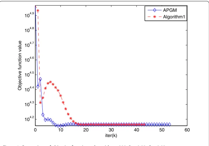
[image:10.595.139.452.315.496.2]Figure 1 Comparison of objective function value withn= 200,Rr= 0.02,Cr= 0.02.
Figure 2 Comparison ofrmsSwithn= 200,Rr= 0.02,Cr= 0.02.
To better observe the convergence and performance of our algorithm, we plot the evo-lutions of the objective function value in Figure ,rmsSin Figure andrmsLin Figure ,
respectively. Plots in these figures indicate that the root mean squares ofSandLdecrease gently at first. However, when approaching the recursion terminal condition, the rmsS
andrmsLin Algorithm decrease more rapidly than APGM. In other words, Algorithm
Figure 3 Comparison ofrmsLwithn= 200,Rr= 0.02,Cr= 0.02.
6 Conclusions
For solving the SPCP problem (.), we proposed a new algorithm based on the PPA in this paper. The global convergence of our algorithm is established. Then the computa-tional results indicate that our algorithm achieves comparable performance with APGM. In certain circumstances, our algorithm can get better results than APGM.
Competing interests
The authors declare that they have no competing interests.
Authors’ contributions
All the authors contributed equally. All authors read and approved the final manuscript.
Acknowledgements
The work is supported in part by the Natural Science Foundation of China Grant 71401176 and the Natural Science Foundation of Jiangsu Province Grant BK20141071.
Received: 3 December 2014 Accepted: 17 April 2015
References
1. Aybat, NS, Goldfarb, D, Ma, S: Efficient algorithms for robust and stable principal component pursuit problems. Comput. Optim. Appl.58(1), 1-29 (2014)
2. Candès, EJ, Li, X, Ma, Y, Wright, J: Robust principal component analysis? J. ACM58(3), 11 (2011)
3. Zhou, Z, Li, X, Wright, J, Candes, E, Ma, Y: Stable principal component pursuit. In: Information Theory Proceedings (ISIT), 2010 IEEE International Symposium on, pp. 1518-1522. IEEE Press, New York (2010)
4. Ma, S: Alternating proximal gradient method for convex minimization. Preprint (2012)
5. Aybat, NS, Iyengar, G: A unified approach for minimizing composite norms. Math. Program.144(1-2), 181-226 (2014) 6. Tao, M, Yuan, X: Recovering low-rank and sparse components of matrices from incomplete and noisy observations.
SIAM J. Optim.21(1), 57-81 (2011)
7. Aybat, NS, Goldfarb, D, Iyengar, G: Fast first-order methods for stable principal component pursuit (2011). arXiv:1105.2126
8. He, B, Yuan, X: On the direct extension of ADMM for multi-block separable convex programming and beyond: from variational inequality perspective
9. He, B, Yuan, X, Zhang, W: A customized proximal point algorithm for convex minimization with linear constraints. Comput. Optim. Appl.56(3), 559-572 (2013)
11. Boyd, S: EE364b Course Notes: Sub-Gradient Methods. Stanford University, Stanford, CA (2010)
12. Martinet, B: Brève communication. Régularisation d’inéquations variationnelles par approximations successives. ESAIM: Math. Model. Numer. Anal.4(R3), 154-158 (1970)
13. Rockafellar, RT: Augmented Lagrangians and applications of the proximal point algorithm in convex programming. Math. Oper. Res.1(2), 97-116 (1976)
14. Ma, F, Ni, M, Zhu, L, Yu, Z: An implementable first-order primal-dual algorithm for structured convex optimization. Abstr. Appl. Anal.2014, Article ID 396753 (2014)
15. Boyd, S, Parikh, N, Chu, E, Peleato, B, Eckstein, J: Distributed optimization and statistical learning via the alternating direction method of multipliers. Found. Trends Mach. Learn.3(1), 1-122 (2011)
16. Chen, C, He, B, Ye, Y, Yuan, X: The direct extension of ADMM for multi-block convex minimization problems is not necessarily convergent. Math. Program., 1-23 (2014)
17. Ma, S, Goldfarb, D, Chen, L: Fixed point and Bregman iterative methods for matrix rank minimization. Math. Program.
128(1-2), 321-353 (2011)
18. Cai, J-F, Candès, EJ, Shen, Z: A singular value thresholding algorithm for matrix completion. SIAM J. Optim.20(4), 1956-1982 (2010)
19. Parikh, N, Boyd, S: Proximal algorithms. Found. Trends Optim.1(3), 123-231 (2013)