Table of contents
1 INTRODUCTION ... 3
1.1 MACHINE TRANSLATION ... 3
1.2 SMT,ALIGNMENT AND PREPROCESSING ... 5
1.3 OVERVIEW OF FURTHER CHAPTERS ... 8
2 STATISTICAL MACHINE TRANSLATION ... 9
2.1 BASIC THEORY ... 9
2.2 LANGUAGE MODELING ... 10
2.3 TRANSLATION MODELING ... 12
2.4 ALIGNMENT ... 14
2.5 THE EXPECTATION MAXIMIZATION ALGORITHM ... 15
2.6 GIZA++ ... 18
2.7 PARAMETER ESTIMATION ... 20
3 PREPROCESSING ... 24
3.1 TOKENIZATION AND SENTENCE ALIGNMENT ... 24
3.2 STEMMING ... 24
3.3 NAMED ENTITY RECOGNITION USING CONDITIONAL RANDOM FIELDS... 25
3.4 NER FOR SMT ... 28
3.5 NER ALGORITHMS FOR BILINGUAL DATA ... 29
3.6 UPPERCASE AND LOWERCASE ... 31
4 EXPERIMENTS AND EVALUATION ... 32
4.1 THE EUROPARL PARALLEL CORPUS ... 32
4.2 ALIGNMENT ERROR RATE ... 32
4.3 PRECISION, RECALL AND F1-SCORE ... 34
4.4 BASIC EXPERIMENTS ... 35
4.5 EXPERIMENTS ON BILINGUAL DATA ... 36
5 EXPERIMENTAL RESULTS ... 37
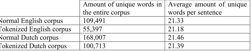
5.1 TOKENIZATION ... 37
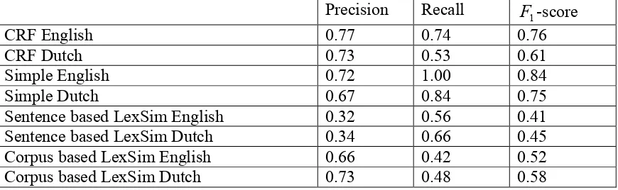
5.2 NAMED ENTITY RECOGNITION ... 37
5.3 STEMMING ... 39
6 REVIEW AND CONCLUSIONS ... 40
6.1 PREPROCESSING EFFECTIVENESS ... 40
6.2 USING BILINGUAL DATA FOR PREPROCESSING ... 41
6.3 FUTURE RESEARCH... 41
7 REFERENCES... 43
1
Introduction
1.1
Machine translation
Machine Translation (MT) is the translation of text from one human language to another by a computer. Computers, like all machines, are excellent at taking over repetitive and mundane tasks from humans. As translating long texts from one language to another qualifies as such a task, Machine Translation is a potentially very economic way of translation. Unfortunately natural languages are not very suitable for processing by a machine. They are ambiguous, illogical and constantly evolving, qualities that are difficult to handle with a machine. This makes the problem of Natural Language Processing, and by extension MT, a difficult one to solve.
A theoretical method that can analyze a text in a natural language and decipher its semantic content can store this semantic content in a language-independent representation. From this representation, another text with the same semantic content can be generated in any language for which exists a generation mechanism. Such an MT architecture would provide high quality translations, and be modular; a new language could be added to the pool of inter-translatable languages simply by developing an analysis and generation method for that language.
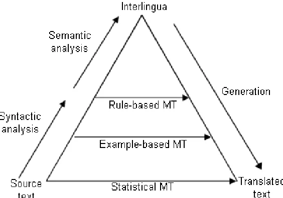
[image:3.595.154.436.477.675.2]Unfortunately this method does not exist. Some existing MT attempts to approach it to a degree, but as long as semantic analysis remains an unsolved problem in the field of Natural Language Processing there can be no true language independent representation. Figure 1 shows the Machine Translation Pyramid, which is a schematic representation of the degree of analysis performed on the input text. The MT method described in these paragraphs is at the top of the pyramid.
Figure 1.The Machine Translation Pyramid, which is an indication of the level of syntactic and semantic analysis performed by various MT methods.
Rule-based Machine Translation
Rule-based MT is a method that focuses on analyzing the source language by syntactic rules. It typically creates an intermediary, symbolic representation from that analysis that represents the content of the text, and then builds a translation from the intermediary representation. In the Machine Translation Pyramid (figure 1), this method is highest up of all the existing MT varieties. It can do syntactic analysis, but since semantic analysis is still an unsolved problem, there is still a need for language-specific translation steps.
Rule-based MT is one of the most popular methods for practical use. Well known rule-based systems include Systran and METEO [1]. Systran was fairly successful, being utilized for a time by both the United States Air Force and the European Union Commission. The system was never abandoned, as today it is used in Altavista’s Babelfish and Google’s language tools. METEO is a system developed for the purpose of translating weather forecasts from French to English, and was used by Environment Canada. It continued to serve its purpose until 2001.
The main advantage to this method of translation is that it works fast. A translation can be produced within seconds, which makes it an attractive method for the casual user. However, the translations produced by Rule-based MT tend to be of poor quality, as Rule-based MT deals poorly with ambiguity.
Example-based Machine Translation
Example-based Machine Translation operates on the philosophy that translation can be done by analogy. An Example-based Machine Translation system breaks down the source text into phrases, and translates these phrases analogous to the example translations it was trained with. New sentences are created by substituting parts of a learned sentence with parts from other learned sentences. This basic principle is explained in a paper by Nagao [2]. In the Machine Translation Pyramid (figure 1), this method is lower than Rule-based MT, because there is little in the way of analysis of the text.
There have been few commercially used example-based translation systems, but the techniques involved are still being researched. A recent proposal for an Example-based MT system was submitted by Sasaki and Murata [3].
The advantage of Example-based MT is that it can produce very high-quality translations, as long as it is applied to very domain-specific texts such as product manuals. However, once the texts become more diverse, the translation quality drops quickly.
Statistical Machine Translation
With advances in statistical modeling the translation quality of SMT systems has risen above that of alternative methods. A paper by Alshawi and Douglas shows this difference in performance [4]. However, the drawback of this method of MT is that it requires massive amounts of processing time and training material to produce a translation. This makes it unsuitable for time-critical applications. Furthermore, SMT is not very effective for language pairs that have little training data available.
In the Machine Translation Pyramid (figure 1), SMT is all the way at the bottom. This reflects the fact that SMT does not syntactically or semantically analyze the input text at all. It simply uses statistics obtained during model training to find a sequence of words it deems the best translation.
Two well-known SMT systems include Moses and Pharaoh. In addition there exists a variety of other systems that focus on components of an SMT system, such as language model trainers and decoders.
1.2
SMT, Alignment and preprocessing
This thesis will investigate preprocessing methods for SMT, in an attempt to find ways to increase the performance of this method of MT. Before we can go into the details of preprocessing we must introduce the workings of SMT.
SMT translates based on information it has trained from example translation data. This example translation data takes the form of a parallel corpus. Such a corpus consists of two texts, each of which is the translation of the other. In this work, this corpus is the Europarl corpus [5], which is freely available for the purposes of SMT research.
By statistically analyzing such parallel corpora, one can estimate the parameters for whatever statistical models one chooses to employ (see Brown et al [6] and Och and Ney [7]).
The trained statistical models are then used by the system to calculate the sentence that has the highest probability of being the translation of the input sentence. The part of the system that does this is called the decoder. Decoding is a difficult problem that is the subject of much research, but it falls outside the scope of this thesis. It is important to note, however, that the performance of the decoder is a function of the quality of the statistical models. Preprocessing on the training data can help improve model quality and by extension the performance of an SMT system.
The sentence-level alignment refers to the way the sentences in the corpus are sequenced. If a given sentence in one half of the parallel corpus is in the same sequential position as a sentence in the other half of the corpus, then those sentence are said to be a sentence pair. If the sentences in a sentence pair are translations of each other, those sentences are said to be aligned. In order to train an SMT system, one requires a parallel corpus the sentences of which are properly aligned. In the remainder of this thesis, we will assume the training data has a correct sentence-level alignment.
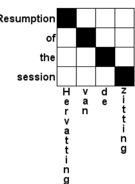
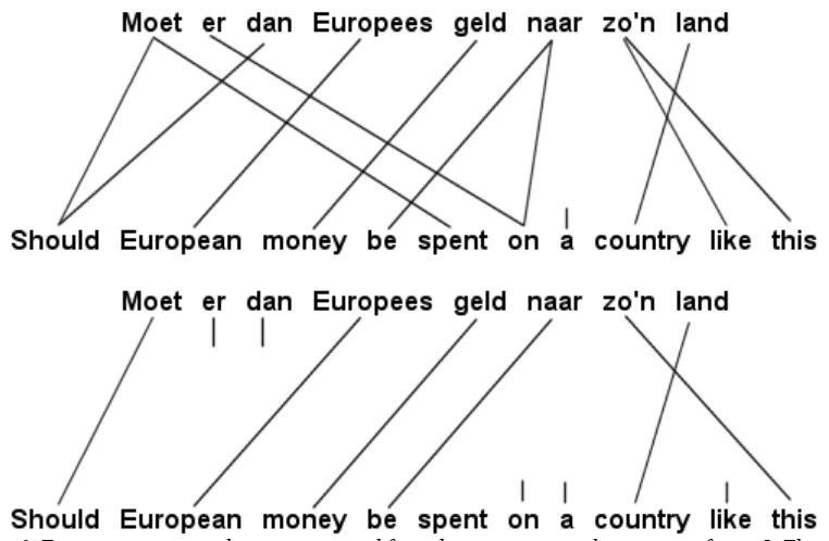
[image:6.595.227.375.281.354.2]Following Och and Ney [8], the word-level alignment is defined as a subset of the Cartesian product of the word positions. This can be visualized by printing a sentence pair and drawing lines between the words. Such a visualization is given in figures 2 and 3. Both visualizations will be used in the remainder of this thesis.
Figure 2 An example of a graphical representation of an alignment on a sentence pair. Words connected by a line are considered to be translations of each other.
Figure 3 The same alignment as shown in figure 2, represented as a subset of the Cartesian product of the word positions.
As is explained in more detail in chapter 2, a word-level alignment is essential for training the statistical models. As training data does not contain a word-level alignment from the get-go, such an alignment must be created by the system.
[image:6.595.235.368.386.567.2]with an alignment that has a low perplexity. Perplexity is a measure of how complex an alignment is. To give a simple example where we only consider word mapping, alignments in which words are mapped to multiple other words will have a higher perplexity than alignments that have few word mappings. The example in figures 2 and 3 has exactly one word associated with each word in the source language, and therefore has a low perplexity.
Perplexity will be formally introduced in chapter 2.
When creating a word-level alignment, a lot depends on the quality of the corpus itself. Things such as spelling errors, missing words or sentences, garbage and mistranslations may negatively influence the accuracy of the alignment, which in turn may negatively affect the translation models that are trained from the alignment. To minimize these negative influences, the corpus can be adjusted prior to the alignment step. Spelling errors can be corrected or simply tokenized away. Incomplete sentence pairs can be removed, as can garbage such as punctuation or formatting codes. It is tasks such as these that are performed by preprocessing.
In addition to eliminating elements that reduce the corpus’ quality, preprocessing can analyze the corpus, often on a semantic level, thereby stimulating a certain tendency in the creation of the word-level alignment. For example, number tagging can ensure that numbers will be aligned to other numbers. For detailed descriptions of preprocessing steps that are relevant in this thesis, refer to chapter 3.
Previous research into preprocessing steps includes work by Habash and Sadat [9], who investigated the effect of preprocessing steps on SMT performance for the Arabic language. Research into preprocessing for automatic evaluation of MT has also been done by Leusch et al [10].
The goals of this work are twofold.
Firstly, it investigates the impact of preprocessing on the performance of SMT training, if the preprocessing is applied to both halves of a parallel corpus. The objective is to judge whether such preprocessing steps are a useful addition to a typical training process. The preprocessing methods examined in this thesis are Stemming, Tokenization and Named Entity Recognition.
1.3
Overview of further chapters
Chapter 2 will give an outline of the SMT theory underlying the experiments. It describes the basic SMT theory, which is later used to explain how preprocessing steps can influence the performance of an SMT system.
Chapter 3 describes the theoretical foundations of the experiments performed. It introduces the techniques involved in the preprocessing steps and explains their working.
Chapter 4 is a description of the experimental setup. It lists the experiments that were performed as well as a predicted result, along with a motivation.
Chapter 5 will show the results of the experiments and provide an explanation as to what they mean and how they reflect the impact of the preprocessing steps.
2
Statistical machine translation
To understand why changing certain properties of a corpus can have an influence on the accuracy of an SMT system, it is important to understand how an SMT system works. An SMT system can roughly be considered as a training process and a decoding process. Because preprocessing has its effect during the training process, this chapter will focus on that and forego a detailed explanation of the decoding process.
2.1
Basic theory
MT is about finding a sentence e that is the translation of a given sentence f . The
identifiers f and e originally stood for French and English because those were the
languages used in various articles written on the subject (Brown et al [6], Knight [11]). This thesis deals with Dutch and English, but will adhere to the convention.
SMT considers every sentence e to be a potential translation of sentence f . Consider
that translating a sentence from one language to another is not deterministic. While a typical sentence can usually only be interpreted in only one way when it comes to its meaning, the translation may be phrased in many different ways. In other words, a sentence can have multiple translations. For this reason, SMT does not, in principle, outright discard any sentence in the foreign language. Any sentence is a candidate. The trick is to determine which candidate has the highest probability of being a good translation.
For every pair of sentences (e, f) we define a probability P(e| f) that e is the
translation of f . We choose the sentence that is the most probable translation of f by
taking the sentence e for which P(e| f) is greatest. This is written as:
) | ( e Argmax
f e
P (1)
SMT is essentially an implementation of the noisy channel model, in which the target language sentence is distorted by the channel into the source language sentence. The target language sentence is “recovered” by reasoning about how it came to be by the distortion of the source language sentence. As the first step, we apply Bayes’ Theorem
to the formula given above. Because P(f) does not influence the argmax calculation, it
can be disregarded. The formula then becomes:
) | ( e Argmax
f e
P = ( ) ( | )
e Argmax
e f P e
P (2)
The highest probability that e is the translation of f has been expressed in terms of the
probability of e a priori and the probability of f given e. At first glance this does not
appear to be beneficial. However, the introduction of factorP(e) lets us find translations
all, every e is a potential translation of f . It isn’t zero even if e is complete gibberish. In effect, this means that some of the probability mass is given to translations that are ill-formed sentences – a sizable portion of the probability mass, in fact. The probability
) (e
P compensates for this. It is called the language model probability. The language
model probability can be thought of as the probability that e would occur. As gibberish
is less likely to occur than coherent, well-formed sentences, P(e) is higher for the latter
than for the former. The probability P(f |e)is called the translation model probability.
The translation model probability is the probability that the sentence e has f as its
translation. Evidently the product P(e)P(f |e) will be greatest if both P(e) and
) |
(f e
P are high – in other words, if f is a translation of e and if e is a good sentence.
It is especially P(f |e) that is of interest for this thesis. As stated in the introduction, preprocessing affects the word-level alignment that the system creates on a corpus, and
the word-level alignment is used to estimate models that are used to calculate P(f |e).
) (e
P gives statistical information about a single language, and as such is not determined
from the alignment. Often, language models are trained separately from translation models, on different data.
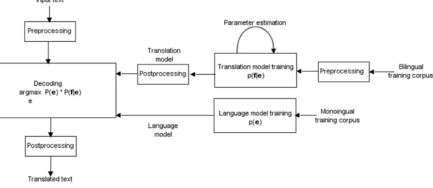
[image:10.595.71.518.421.615.2]Figure 4 is a graphical representation of the above. This figure shows a basic SMT system, including preprocessing for the translation model training.
Figure 4A more detailed schematic of an SMT system’s architecture. Note that the language model is trained from separate (monolingual) training data.
As will be clear, a good SMT system requires a good language model as well as a good translation model. The remainder of this chapter describes how one may obtain such models.
The language model P(e) is largely determined by the training corpus that was used to train the language model. The more similar the sentence is to the raining data, the higher its P(e) score will be.
An important part of this probability is the “well-formedness” of the sentence. A sentence that is grammatically correct is a well-formed sentence, whereas a sentence that is a mere collection words that bear no relation to each other is ill-formed.
While well-formedness is important, it is not all that matters for the language model probability. The words used in the sentence also have their impact. If a sentence uses
many uncommon words, it may be given a lower P(e) score than a sentence that only
uses more common words. For example, a sentence that uses the words “mausoleum”,
“nanotechnology” and “comatose” together may be given a lower P(e) score than a
sentence that uses the words “cooking”, “house” and “evening” together. Of course, if the training corpus was largely on the subject of people being held comatose in a mausoleum by means of nanotechnology, the opposite might be true, as the former sentence would be using common words given that training corpus.
The language model can be trained by simple counting. Training requires a training corpus, preferably as large a corpus as possible, which contains sentences in the language for which the language model is being trained. From this corpus a collection of n-grams is constructed. An n-gram is a fragment of a sentence that consists of n consecutive words. For example, the sentence “Resumption of the session” contains five 2-grams: “<s> Resumption”, “Resumption of”, “of the”, “the session” and “session <s>”, where <s> and </s> indicate the absence of a word at the start and the end of the sentence, respectively.
The n-grams can then be assigned probabilities as follows:
) ... ( #
) ... ( # ) ... | (
1 0
0 1
0
− − =
n n n
n
X X
X X X
X X
P (3)
Where
X
is a word in the sentence, X0...Xnis an n-gram and # is the number ofoccurrences of in the corpus. Any sentence that can be constructed from the n-grams
that the system has learned can be assigned a P(e) that is a function of the probabilities
However, this isn’t sufficient. A sentence that cannot be built out of learned n-grams will be given a probability of zero, which means the system will not be able to generate those sentences. As training data is finite and the number of possible sentences is not, it will always be possible to construct a sentence that has one or more n-grams that do not occur in the training data, no matter how large the training corpus is. Therefore, we employ a technique called smoothing, which assigns a nonzero probability to every possible n-gram given the words in the training corpus, even those that don’t actually occur. This allows the system to generate sentences that contain n-grams that weren’t in the training corpus, as long as those n-grams contain known words. There are many possible approaches to smoothing, the most simple being the addition of a very small value to every n-gram that did not appear in the corpus.
There are other methods of building a language model, though the smoothed n-gram method is prevalent. These methods are outside the scope of this thesis. However, it is worth pointing out that Eck et al [12] investigated a method that expands on the n-gram method by adapting the language model to be more domain specific, thereby achieving better results in that domain.
2.3
Translation modeling
The purpose of the translation model is to indicate for a given sentence pair (e, f) the
probability that f is the translation of e. It assigns a probability to each potential
translation of the input sentence, and if the model is any good, better translations will have higher probabilities. Training models that will yield good probabilities is not easy, and in fact a great deal of the research done in the field of SMT is related to translation modeling.
The approach used by the SMT translation models is called string rewriting. It is described in detail by Brown et al [6]. String rewriting essentially replaces the words in a sentence with their translations, then reorders them. While string rewriting cannot explicitly map syntactic relationships between words from the source sentence to the target sentence, it is possible to approximate such a mapping statistically. The upside to this method is that it’s very easy in principle, and it can be learned from available data. This means that as long as appropriate training data is available this method applies to any language pair.
The first parameter is the amount of translated words that are associated with every
source word. This is called the fertility of that word. For example, a word with a fertility
of 3 will have 3 words associated with it as a translation of that word. The fertility for a word is not directly dependent on the other words in the sentence or their fertilities, but as the sum of all fertilities must be equal to the amount of words in the target sentence, fertilities indirectly influence each other by competing for words when estimating the fertility probabilities during model training.
The part of the translation model that decides on the fertility is called the fertility model.
This model assigns to each word ei a fertility
φ
i with probability) | ( i ei
n φ (4)
Secondly, the translation model decides which translation words are generated for each
word in the source sentence. This is called the translation probability, not to be
confused with the translation model probability. More formally, for each word ei the
generation model chooses k foreign words
τ
ik with probability) | ( ik ei
tτ (5)
With 1≤k≤φi
Thirdly, the translation model decides the order in which these translated words are to
be placed. This part of the translation model is called the distortion model. The
distortion model chooses for each generated word
τ
ik a positionπ
ik with probability) , , |
( i l m
d πik (6)
Where l is the amount of words in the source sentence and m is the sum of all
fertilities.
Finally, the translation model causes words to be inserted spuriously. To understand this, consider that sometimes, words that appear in a translation may not be directly generated from a word in the original sentence. For example, a grammatical helper word that exists in one language may have no equivalent in the other language, and will therefore not be generated by any of the words in that language. For this reason, all sentences are assumed to have a NULL word at the start of the sentence. This NULL word can have translations like any other word, which allows words without a
counterpart in the original sentence to be generated. This is called spurious insertion.
Every time a word is generated normally in the target sentence, there is a probability that a word is generated spuriously. This probability is denoted with
1
The probability p0 is the probability that spurious generation does not occur, given by
1
0 1 p
p = − (8)
In the following section we will see how these parameters can be turned into the
translation model probability P(f |e) that we’re looking for, by means of a word-level
alignment.
2.4
Alignment
An actual translation model is trained from a word-level alignment. The parameters described in the previous section can be estimated from a word-level alignment.
) |
( e
n φ for a certain e and φ can be obtained simply by checking the word-level
alignment on the entire corpus, counting all the occurrences that eis aligned to exactly
φ words in the foreign language, then dividing this count by the amount of probabilities
n in the translation model.
n e e n # ) | ( # ) |
(φ = φ (9)
) |
( e
tτ for a certain
τ
and e can be obtained by counting how many words aregenerated by all occurrences of e in the alignment and then dividing the amount of
τ
by the total count.
) | ( # ) | ( # ) | ( e x e e
t τ = τ (10)
Where x means “any word”.
) , , |
( i l m
d π for a certain
π
,i,l and m can be obtained by counting the occurrences of) , , |
(π i l m and dividing it by the count of all occurrences of (j|i,l,m), with j=1...m.
) , , | ( # ) , , | ( # ) , , | ( m l i j m l i m l i
1
p can be obtained by looking at the foreign corpus. This corpus consists of N words.
We reason that M of these N words were generated spuriously, and that the other
M
N − words were generated from English words. M can be obtained from the
word-level alignment by counting the occurrences of translation parameter (x|"NULL"). This
leads to the value for p1:
M N
M p
− =
1 (12)
The above shows that it is vitally important for the word-level alignment to be as accurate as possible. The ideal scenario is that every word in a sentence is aligned to a word that is a translation of that word, or if there is no translation of that word available in the translation sentence, that it not be aligned to another word at all.
In practice, prefabricated word-level alignments do not exist. It falls to the SMT system training process to estimate one from the sentence-aligned corpus. Because the trainer has no knowledge of the languages involved at all, it must determine which alignment is the best one based on patterns that exist in the corpus. For this purpose we employ the Expectation Maximization (EM) algorithm (Al-Onaizan et al [13]).
2.5
The Expectation Maximization algorithm
EM is an iterative process that attempts to find the most probable word-level alignment on all sentence pairs in the parallel corpus. It attempts to find patterns in the corpus by statistically analyzing the component sentence pairs, and considers alignments that conform to these patterns to be better than alignments that don’t. This is why preprocessing on the corpus has an effect on the overall translation model quality. By modifying the corpus we modify certain patterns, with the intent to direct the EM algorithm produce a better alignment.
In creating a word-level alignment on a sentence-aligned corpus, we consider that each sentence pair has a number of alignments, not just a single one. Some of these alignments we may consider “better” than others. To reflect this, we introduce alignment weights. An alignment with a higher weight is considered better than an alignment with a lower weight. The sum of the alignment weights for all alignments on a sentence pair is equal to 1. There weights will help us estimate the translation model
parameters by collecting fractional counts over all alignments. The basic method is the
The question arises where these alignment weights come from. Let us express these
weights in terms of alignment probabilities. The probability of an alignment on a
sentence pair (e, f)is the probability that the alignment would occur given that sentence
pair. We write this probability as
) , |
(a e f
P (13)
Where a is the alignment. We can use the definition of conditional probability to
rewrite this probability as
) , |
(a e f
P = ) , ( ) , , ( f e P f e a P (14)
Because e is statistically independent of both f and a, we can write
) , |
(a e f
P = ) ( ) | ( ) ( ) | , ( e P e f P e P e f a P (15)
After dividing out P(e) we end up with
) , |
(a e f
P = ) | ( ) | , ( e f P e f a P (16)
It is easy to see that taking the sum over a of all probabilities P(a, f |e)is the same as
) |
(f e
P :
) |
(f e
P =
∑
a
e f a
P( , | ) (17)
In other words:
) , |
(a e f
P =
∑
a e f a P e f a P ) | , ( ) | , ( (18)Finally, P(a, f |e)is calculated as follows:
! 1 ) , , | ( ) | ( ) | ( ) | , ( 0 0 1 1 1 1 2 0 0
0 0 0
φ φ
φ φ
φ φ φ
Where
e is the source sentence
f is the foreign sentence
a is the alignment
i
e is the source word in position i
j
f is the foreign word in position j
l is the number of words in the source sentence
m is the number of words in the foreign sentence
j
a is the position in the source language that connects to position j in the foreign
language in alignment a
aj
e is the word in the source sentence in position aj
i
φ
is the fertility for the source word in position i given alignment a1
p is the probability that spurious insertion occurs
0
p is the probability that spurious insertion does not occur
Note that, in deducing the formula for P(a|e, f) , we introduced a formula for
calculating P(e| f) (formula 17). Remember that this is the translation model
probability that we ultimately aim to establish by training the translation models.
In summary, the alignment probability P(a|e, f) can be expressed in all the translation
model parameters. As we already asserted, these translation model parameters can be calculated given the alignment probability. If we have one, we can compute the other. Needless to say we start out with neither, which presents a problem. This is often referred to the chicken-and-egg problem. We will need a method for bootstrapping the training, and Expectation Maximization is exactly that.
EM searches for an optimization of numerical data. As EM iterates it will produce alignments it considers “better”. In this context, “better” means a lower perplexity. In the introduction, perplexity was described as a measure of complexity. With the theory described in this section, we are ready for a more formal definition:
N e f P( |) log
2− (20)
Remember that P(f |e) can be expressed in terms of P(a, f |e)(equation 14). N is the
amount of words in the corpus. The higher P(f |e) is, the lower the perplexity will be.
) |
(f e
P is higher if the parameters that make up P(a, f |e) have higher values. Finally,
the parameters will have higher values when their fractional counts – over the entire corpus – are high. Because simple relationships between words will show up more often than complex ones, alignments with such simple relationships will yield higher parameter values.
What EM does is find the lowest perplexity it can. Each iteration lowers perplexity. However, because perplexity is a measure over a product of the parameters, the EM algorithm is only guaranteed to find a local optimum, rather than the global optimum. The optimum it finds is partly a function of where it starts searching, or to put it in other words, what parameter values it starts with.
There are several EM algorithms imaginable. For example, there could be an EM algorithm that simplifies the translation model by ignoring fertility probabilities, probabilities for spurious insertion and distortion probabilities. This EM algorithm will only optimize perplexity in terms of the translation probability parameter. As there is only one factor to optimize, this EM algorithm will be guaranteed to find the global optimum for its perplexity. This EM algorithm exists, and it is the EM algorithm used in IBM Model 1.
2.6
GIZA++
In practice the alignment is generated by a program called GIZA++. GIZA++ is an extension of GIZA, which is an implementation of several IBM translation models. In addition to the IBM models, GIZA++ also implements Hidden Markov Models (HMMs). By request this thesis acknowledges Franz Josef Och and Hermann Ney for GIZA++. The theory of their implementation is described in [8].
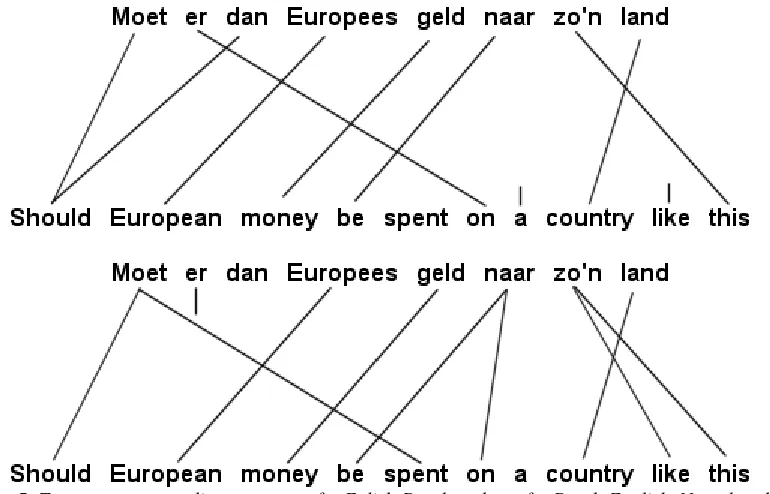
Figure 5.Two one-to-many alignments, one for Enlish-Dutch and one for Dutch-English. Note that these alignments are not optimal. Some errors exist, such as the alignment of “naar” to “be”.
To achieve a many-to-many alignment from GIZA++ it is necessary to produce two one-to-many alignments, one for each translation direction, and combine them into a single many-to-many alignment. This process is referred to as symmetrization. There are two methods of symmetrization used in these experiments: Union and Intersection symmetrization.
Union symmetrization assumes that any alignment the two one-to-many alignments do not agree on should be included in the many-to-many alignment. Formally:
2
1 OTM
OTM
MTM A A
A = ∪ (21)
Intersection symmetrization assumes that any alignment the two one-to-many alignments do not agree on should be discarded. Words that no longer have any alignment after symmetrization are aligned to NULL. Formally:
2
1 OTM
OTM
MTM A A
A = ∩ (22)
Figure 6. Two many-to-many alignments created from the one-to-many alignments in figure 5. The upper figure is the Union alignment and the lower figure is the Intersection alignment.
2.7
Parameter estimation
When optimum perplexity has been achieved, the alignment with the highest probability is called the Viterbi alignment. The Viterbi alignment found by Model 1 when starting off with uniform parameter values may be a very bad alignment. For example, all words could be connected to the same translation word. Model 1 has no way of knowing that this is not a probable alignment, because it ignores all the parameters that show this improbability, such as the fertility parameter. However, the Model 1 Viterbi alignment can be used as the starting position for more complex EM algorithms. More complex algorithms have more parameters that weigh into the perplexity, and they are not guaranteed to find a global optimum. From the most probable alignment given a local optimum we can get a new set of parameters. This new set of parameters can then be fed back to Model 1, which may find a new Viterbi alignment as a result of its new starting parameters.
This last part is an important aspect of translation model training. By using the parameters from a training iteration of one model, we can start a new training iteration, with that same model or with a different one, which will hopefully yield improved
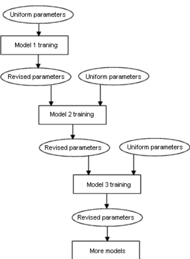
parameter values. This process is called parameter estimation. A simple, schematic
Figure 7.A schematic representation of the parameter estimation process. The models can each be trained a number of times, taking the results from the previous iteration as the starting point for the new
iteration. When a model estimates parameters that were not estimated by a previous model, it starts the first training iteration with uniform values for those parameters.
There is one practical problem with starting the parameter estimation process. Recall
that P(a|e, f)can be expressed in terms of P(a, f |e)(see formula 18). In the Model 1
EM algorithm, the denominator of that formula,
∑
a
e f a
P( , | ), can be written as
∑∏
=
a m
j
aj j e
f t
1
) |
( (23)
As is implied by this formula, the EM algorithm needs to enumerate over every
alignment in the corpus. In a corpus of N words in language e and M words in
language f , the amount of alignments is equal to
M
N 1)
( + (24)
To illustrate, in a single sentence pair with 20 words in each sentence, the amount of
alignments is 26
10
2.78⋅ . For a corpus with 120,000 sentence pairs the amount of
As formula 21 sums over a product that contains independent elements, we can factor out the elements independent to the product and take the product over the independent element of the sum of the factored expression:
∏∑
= −
m
j l
i
i j e
f t
1 0
) |
( (25)
With this formula, the amount of alignments to be enumerated to get the fractional counts for all alignments is equal to
M
N +1• (26)
This formula has a quadratic order of magnitude, whereas formula 22 has an exponential order. To illustrate, consider again the single sentence pair with 20 words in each sentence. The amount of alignments to enumerate is now only 420.
The above means that we can enumerate all the alignments for IBM Model 1 within reasonable time, and therefore find the Viterbi alignment. The same is true for IBM Model 2, which is like Model 1, but handles distortion probabilities as well as translation probabilities. Unfortunately, this manner of simplification cannot be performed for complex models like IBM Model 3, and so we cannot find their Viterbi
alignment in reasonable time. However, there is a technique called hill climbing that can
be used to find the (local) optimum for such models. Hill climbing takes for every sentence pair a single alignment to start with. A good place to start would be the Model 2 Viterbi alignment. The model then makes a small change to the alignment, for example by moving a connection from one position to another position close by. Then the model computes the perplexity for the new alignment. This can be done fairly quickly with formula 19. If the new alignment is worse, it is discarded. If it is better, it replaces the old alignment. The model repeats this process until no better alignment can be found by making a small change. The alignment the model ends up with is considered the Viterbi alignment for this model, even though there is no guarantee that the alignment is, in fact the best alignment given the current parameter values. From this “Viterbi” alignment and a small set of alignments that are “close” to it we can collect fractional counts and estimate a new set of parameters. This new set of parameters can be used as the starting point for a new training iteration or, if no more
training is deemed necessary, to calculate the final P(f |e).
3
Preprocessing
Preprocessing is literally to process something before it is processed by something else. In computer science a preprocessor is a program that processes its input data to produce output that is used as input to another program. In the specific context of these experiments the output data of the preprocessors serves as the input data for GIZA++. This chapter gives an overview of the preprocessing techniques used in the experiments.
3.1
Tokenization and sentence alignment
Following Webster and Kit [14], tokenization is defined as a type of preprocessing that decomposes parts of a given text into more basic units. An example of tokenization on English is decomposing the contraction “it’s” into “it is”.
The tokenization employed in these experiments is limited to the removal of punctuation and words that do not bear any semantic significance, such as corpus markup.
Tokenization on punctuation is a trivial task in itself. However the scripts that are included with the Europarl corpus take a slightly more involved approach, making use of a list on non-breaking prefixes. These non-breaking prefixes indicate words that do not mark the end of a sentence when encountered with a period. The list is used not only in tokenization but also for sentence alignment, and later it will be used during Named Entity Recognition as well. Europarl includes a list of non-breaking prefixes for English, but not for Dutch.
Although a Dutch list is not required to remove punctuation on the corpus, the list can also be used during the sentence-alignment of the text. If no suitable list is found for a language, the sentence alignment script falls back to English. This can result in a bad sentence alignment, which is effectively useless as a base to train statistical translation models.
A list of Dutch non-breaking prefixes is shown in Appendix A.
3.2
Stemming
In the context of Natural Language Processing, a word’s stem is taken to be the first part of that word, stripping off any trailing letters that might constitute inflections, conjugations or other modifiers to the word. It is important to note that the stem thus generated is not necessarily the same as the morphological root of that word. In stemming for NLP, it is usually sufficient that related words map to the same stem, even if this stem is not in itself a valid root.
Example 8 illustrates the result of stemming on a small selection of words.
consist consisted consistency consistent consistently consisting consists
consist consist consist consist consist consist consist knock
knocked
knock knock knocker
knockers
knocker knocker
Example 8. Examples of stemming applied to a few English words and their variations.
The stemming algorithm used in most NLP related tasks is the Porter stemmer, or a stemmer derived from the Porter stemmer. The stemmer used in this experiment is no exception; the stemmer used is the Porter2 stemmer, which is a slightly improved version of the Porter stemmer. The Porter stemming algorithm is described by Porter et al [15].
Because stemming directly changes the corpus, it requires a postprocessing step to restore the words in the corpus to their original forms once the alignment has been computed, as estimating the translation model parameters from a stemmed corpus would not result in a very good SMT system.
3.3
Named Entity Recognition using Conditional Random Fields
Named Entity Recognition (NER) is a subtask of information extraction that seeks to locate and classify Named Entities (NEs), which are expressions that refer to the names of persons, organizations, locations, expressions of times, quantities, monetary values, percentages, etc.
CRFs are conditional probabilistic models not unlike HMMs for labeling or segmenting sequential data, such as a plaintext corpus. One of the problems with labeling sequential data is that the data often cannot be interpreted as independent units. For example, an English sentence is bound by grammatical rules that impose long-range relationships between the words in the sentence. This makes enumerating all observation sequences intractable, which in turn means that a joint probability distribution over the observation and label sequences, as would be the case in an HMM, cannot be calculated in reasonable time. On the other hand, making unwarranted independence assumptions about the observation sequences is not desirable either. A solution to this problem is to define a conditional probability given a particular observation sequence rather than a joint probability distribution over two random variables.
Let
X
be a random variable that ranges over observable sequences of words, and letY
be a random variable that ranges over the corresponding sequences of labels, in this case
named entity tags. A CRF defines a conditional probability P(Y|x) given a particular
observed sequence of words x. The model attempts to find the maximal probability
) | (y x
P for a particular label sequence
y
. Let G=(V,E) be an undirected graph suchthat there is a node v∈V corresponding to each of the random variables representing an
element Yv of
Y
. If each random variable Yvobeys the Markov property with respectto G , then (Y,X) is a CRF. The Markov property entails that the model is memoryless,
meaning each next state in the model depends solely on its previous state.
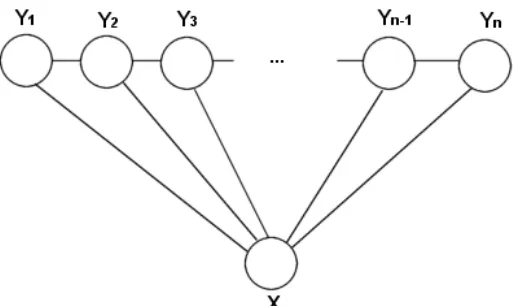
[image:26.595.172.429.456.609.2]While in theory G may have any structure, in practice it always takes the form of a simple first-order chain. Figure 9 illustrates this.
Lafferty et al. [16] define the probability of a particular label sequence y given observation sequence x to be a normalized product of potential functions, each of the form ) ) , , ( ) , , , (
exp(
∑
−1 +∑
k i k k j i i j
jt y y x i
µ
s y x iλ
(27)Where tj(yi−1,yi,x,i)is a transition feature function of the entire observation sequence
and the labels at positions
i
and i−1in the label sequence, and sk(yi,x,i)is a statefeature function of the label at position
i
and the observation sequence. λj andµ
k areparameters that are obtained from the training data. These feature functions take on the values of one of a number of real-valued features. Such features are conditions on the
observation sequence that may or may not be satisfied. For example, a feature b(x,i)
could be = otherwise 0, letter capital a with starts position at word the if 1, ) ,
(x i i
b (28)
A state feature function for this feature could be
= = otherwise 0, IN if , ) , ( ) , ,
( i i
k y i x b i x y s (29)
Similarly, a transition feature function tj(yi−1,yi,x,i)is defined on two states and a feature.
With such features and feature functions, we can write the probability of a label sequence y given an observed sequence x as
) ) , ( exp( ) ( 1 ) , | ( =
∑
j j jF y xx Z x
y
P
λ
λ
(30)Where
) ( 1
x
Z is a normalization factor and Fj(y,x) is the sum over all feature functions,
Given this probability we can calculate the maximal probability by maximizing the logarithm of the likelihood, given by:
∑
∑
+ =
Λ
k j
k k f j
k F y x
x
Z( ) ( , )
1 log )
(
λ
( )λ
( ) ( ) (31)Because this function is defined on the probabilities of local label sequences, we can ensure we get the general label sequence with the highest probability by maximizing this function. It is concave, which ensures convergence to a global maximum.
An NER system that implements CRFs is the Stanford Named Entity Recognizer (Rose Finkel et al [17]), which scored 86.86 F-score on the CoNLL2002 shared task and 92.29 on the CMU Seminar Announcement dataset (these are the highest overall scores only). This system will be used in the CRF NER experiments described in this thesis.
3.4
NER for SMT
An NE is special from the perspective of SMT in the sense that each NE can only have exactly one translation, no more and no less. Though some entities may have more than one name, they are typically indicated with only one of the possible names throughout the use of the language. For example, In English the Belgian town of Bruges is always referred to by that name, though in Dutch the town is invariably referred to by its Dutch name, Brugge. We can say that in this specific example, Bruges in English is the correct translation of Brugge in Dutch, and that any other translation is wrong.
Linguistically speaking NER is aimed towards finding and classifying exactly those words that are indeed NEs, and no others. In tasks such as information retrieval it is important to achieve a high precision and recall under those constraints, because of the semantic significance of the words. In the context of training an SMT system, however, there is a different consideration that comes into play.
3.5
NER algorithms for bilingual data
Sentence pair based lexical similarity
This algorithm tags words as NEs by checking for a lexically similar word in the translation sentence. For each word it calculates the maximum lexical similarity score for that word given all the words in the translation. Lexical similarity is a measure of how closely two words resemble each other. The words “Parlement” and “Parliament”, for example, are lexically quite similar because they have many letters in common. In the experiments, lexical similarity is defined as
) , max( 1
similarity
2
1 N
N D −
= (32)
Where D is the Levenshtein distance (Navarro, [18]) between the two words and N1
and N2 are the lengths of the words.
The Levenshtein distance is a measure about how different the words are in terms of how many elementary operations to one word need to be preformed to obtain the other word. An elementary operation is either the substitution of any letter with a different letter, the addition of a letter at any position in the word or the removal of any letter in the word.
In equation 30, the Levenshtein distance is normalized by the length of the longer of the two words. The reason for this is that the Levenshtein distance only indicates the absolute difference between two sequences. For example, the words “European” and “Europa” have a Levenshtein distance of 2, because it takes 2 elementary operations to obtain one from the other. However, the same can be said for the words “of” and “in”, which are clearly not very lexically similar. By normalizing for word length we obtain a score that gives an indication of how many letters the two words have in common relative to how many are different. An example of this algorithm is shown in example 10.
English: One of the people assassinated very recently in Sri Lanka was Mr Kumar Ponnambalam, who had visited the European Parliament just a few months ago.
Dutch: Een van de mensen die zeer recent in Sri Lanka is vermoord, is de heer Kumar Ponnambalam, die een paar maanden geleden nog een bezoek bracht aan het Europees Parlement.
recently recent
Sri Sri
Lanka Lanka
Kumar Kumar
Ponnambalam Ponnambalam
European Europees
Parliament Parlement
While all NEs in this example have been successfully recognized, note how “recently” and “recent” were also recognized as NEs because they are sufficiently similar. This shows that judging NEs by lexical similarity is prone to false positives.
Corpus based lexical similarity
Corpus based lexical similarity is like sentence based lexical similarity, but it attempts to avoid some of the problems inherent to the sentence based approach.
To combat false positives, the algorithm imposes two conditions on the word pairs. Firstly, a matching word pair must occur at least a certain amount of times in the corpus. Singletons are statistically insignificant, and are even likely to decrease the alignment accuracy. Secondly, the algorithm calculates an occurrence score for each matching word pair. Even if a matching word pair is found, this pair cannot be considered a NE if the component words appear unpaired too often in the text. The NER algorithm will not consider a matching word pair to be a NE pair if its occurrence score is too low.
Formally, for every unique word w and for all sentence pairs (i,j)in the corpus the
occurrence score for that word is calculated as:
∑
∑
∑
+ •
=
j j i
i j i
j i i
w w
w w
w
score (, )
) , min( 2
)
( (33)
Sri Sri
Lanka Lanka
Kumar Kumar
Ponnambalam Ponnambalam
European Europees
Example 11.Lexical similarity NER using minimum occurrence and minimum length constraints.
Note that “Parlement” and “Parliament” are now not recognized as NEs. This can be remedied by reducing the similarity threshold.
Re-classifying unclassified tags
Most of the tagging algorithms described here do not classify the NEs, as the classification is not immediately relevant to the word level alignment. However, classification can help establish a correct alignment.
The re-classification algorithm compares two unclassified tagged corpora to their respective untagged versions and classifies the tags according to the lexical similarity score of the tagged words only. A tagged word that has a lexically identical counterpart in the translation sentence will be marked as <NE_VERBATIM>, a tagged word that is not lexically identical yet lexically similar above a given threshold will be marked as <NE_SIMILAR> and all tagged words that have no lexically similar counterparts will remain unclassified. The expectation is that such a re-classification will lead to a better Alignment Error Rate while not reducing the NER performance.
3.6
Uppercase and lowercase
The sentences in the Europarl corpus are punctuated and capitalized. While punctuation is only markup that benefits a human reader, capitalization can be used to analyze the text from a MT point of view. For example, capitalization might be used to identify named entities, or to facilitate part-of-speech tagging. However, because capitals are also used at the beginning of sentences and sentences can begin with practically any word, a capitalized corpus is inherently more complex than a corpus with the capitals removed.
Capitalization typically is highly language specific. For one thing, it is limited to languages that use the alphabet. And even amongst alphabet-based languages there are often differences. In English it is customary to capitalize the names of days and months, as well as the first person pronoun “I”, while in Dutch this is not the case. In German every noun is capitalized.
4
Experiments and Evaluation
Chapters 2 and 3 provided the theoretical background of an SMT system and (some types of) preprocessing. This chapter describes the data used for the experiments, how the various preprocessing techniques are applied to this data, what the expected effect is on the alignment and how the performance is evaluated.
4.1
The Europarl parallel corpus
The experiments in this thesis were performed on a parallel corpus called Europarl (Koehn, [19]). The corpus is extracted from the proceedings of the European Parliament from April 1996 to December 2001. Most of the sentences are the sentences spoken by the politicians in the Parliament, translated if the speaker was speaking in a language other than the language used in the corpus. The translation was created manually by teams of freelance translators employed by the European Parliament. The sentences cover political debates and procedural conversation between the politicians and the president of the Parliament. In addition, the corpus contains descriptive sentences that indicate non-verbal action taken by the Parliament at large.
The corpus contains about 20 million words in 743,880 sentences per language. The corpus is available in a sentence aligned format.
4.2
Alignment Error Rate
The effectiveness of a preprocessing step can be expressed as the improvement in the alignment that it causes.
To determine how “good” any generated alignment actually is, a point of reference is needed. For this purpose, a reference alignment must be created. This reference alignment represents the “correct” alignment. The alignment created by the system should ideally be identical to this reference alignment. Because the reference alignment must be made manually, it is relatively costly to produce. For that reason, only a small portion of the corpus is used for the reference alignment.
The accuracy of the generated alignments is the degree in which they differ from the reference alignment. This is called the Alignment Error Rate. The Alignment Error Rate is the most important evaluation measure used in this thesis.
The Alignment Error Rate is a measure of how similar two alignments are to each other. The definition of the AER is given by Och and Ney [8]:
S A
P A S A A
P S AER
+ ∪ + ∩ −
=1 | |
) ; ,
( (34)
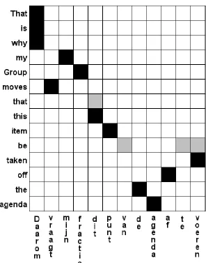
[image:33.595.152.448.282.659.2]Where S is the Sure alignment, P is the Possible alignment and A is the generated alignment for which the AER is being calculated. A Sure alignment is an alignment that is always considered to be correct. A Possible alignment is an alignment that may be correct. Possible alignments can be used to resolve differences in opinion between multiple human aligners. An example of an alignment that combines Sure and Possible alignments is shown in figure 12.
Figure 12.A sentence pair that was aligned using Sure and Possible alignments. The black fields are the Sure alignment and the grey fields are the Possible alignment. While the Possible alignment may seem to be largely in error, it could have been established like this because some human aligners chose to align
The manual alignment used as the reference for the experiments described here only includes Sure alignments, no Possible ones, due limited time and resources. This means that for the purpose of calculating the Alignment Error Rate in this instance, formula 25 should be rewritten as
S A S A A S + ∩ ⋅ − =1 2 ) ; (
AER (35)
Some sentence pairs provide a poor match on the semantic level (and as a result have few words that can be aligned). These sentences contain many words that are aligned to NULL. The AER score for a standard training on these sentences is likely to be low, but the score could increase as a result of preprocessing, because words are properly aligned to NULL.
4.3
Precision, recall and F
1-score
Precision and recall are standard evaluation measures used for many NLP related tasks. In the context of NER, precision is the portion of the words recognized that are in fact
NEs. Recall is the portion of NEs in the text that was successfully recognized. The F1
-score is a measure that combines precision and recall into a single scalar -score.
Precision is defined as
A A M precision # ) ( # ∧ = (36)
Where
M
denotes an NE that was manually tagged andA
denotes an NE that wasautomatically tagged. Classification, if present, is ignored.
Recall is defined as
M A M recall # ) ( # ∧ = (37)
The F1-score is defined as
recall precision recall precision F + ⋅ ⋅ = 2 1 (38)
4.4
Basic Experiments
The following is a list of the preprocessing experiments and the expected effect. The experiments in this section are strictly limited to preprocessing steps that apply to monolingual data.
Tokenization
This is a GIZA++ training on the corpus after tokenization for punctuation. No other tokenization was applied to the corpus. The AER score for this training is considered the baseline. If an AER score is said to improve or worsen, it does so relative to the AER for this training.
Stemming
In this experiment the porter2 stemmer described in section 3.2 was applied to both halves of the parallel corpus. The stemmed corpus was then used to train an alignment, following which a postprocessing step was performed to restore the corpus to its original state.
As stemming reduces the amount of unique words in a corpus, it reduces the complexity of the alignment training task, in the sense that the EM algorithm no longer has to distinguish between morphological variants of words. This will result in a stronger bias towards alignments that align words that were previously morphological variants, which in turn reduces the perplexity of the alignment.
Simple NER
The simple algorithm considers any word that starts with a capital letter an NE, as long as it isn’t at the start of a sentence. It judges the latter condition by checking if the word is the first in the input, and subsequently by checking for a period at the end of the preceding word, excepting those words listed in the list of non-breaking prefixes.
As the name suggests this algorithm is unsophisticated and will likely yield a low performance in terms of precision and recall as well as AER improvement.
Conditional Random Field NER
This is an experiment with a corpus annotated by the CRF NER algorithm. The corpus was annotated using the standard classifier for the Stanford CRF NER implementation, which uses three tag types: <PERSON>, <ORGANIZATION> and <LOCATION>.
4.5
Experiments on bilingual data
These experiments attempt to improve on the performance of the experiments described in section 4.4 by using bilingual information.
NER with sentence based lexical similarity
This experiment uses the lexical similarity algorithm described in section 3.5. Each word is in a given sentence pair is examined for lexical similarity with all words in the other sentence. If a word pair is found which is lexically similar to a sufficient degree, specified by a similarity threshold, that pair is considered an NE pair and will be tagged. In addition a minimum word length may be specified. Words that are smaller than the minimum specified word length will never be considered as part of an NE pair. The minimum word length is a measure to avoid false positives among very short words. Precision may be increased by increasing this parameter, but recall is likely to suffer as a result.
However even by doing so, it is expected that too many non-NE words will be falsely tagged. The AER may not improve much, or even worsen as a result.
NER with corpus based lexical similarity
This is an experiment using the lexical similarity algorithm described in section 3.5, which takes into account occurrence information of word pairs in the corpus. The algorithm tags words based on a lexical similarity threshold as well as an occurrence threshold. The occurrence threshold is a measure to improve precision by disqualifying suspected false positives.
This algorithm is expected to perform substantially better than the sentence based approach in terms of precision. Recall, however, is expected to be roughly the same because the lexical similarity algorithm that judges NEs is identical.
Reclassification of unclassified NER
By reclassifying unclassified NE tags, an attempt is made to ensure that NEs that look the same will always be aligned to one another, rather than unrelated NEs that may be present in the sentence pair.