ISSN: 2334-2366 (Print), 2334-2374 (Online) Copyright © The Author(s). 2014. All Rights Reserved. Published by American Research Institute for Policy Development
Simulation and Numerical Modeling of a Rectangular Patch
Antenna Using Finite Difference Time Domain (FDTD) Method
El Hajibi, Y.1 & El Hamichi, A.1
Abstract
This work is to apply the numerical method of Finite Difference Time Domain ( FDTD ) for modeling a rectangular patch antenna via a MATLAB code using UPML formulation for absorption boundary conditions. Reflection coefficient andinput impedance of this antenna are determined and compared with simulation results by the HFSS soft.
Keywords: FDTD method, Uniaxial Perfectly Matched Layer formulation (UPML), Reflection coefficient S11 and input impedance Zin of the antenna
Introduction
Since its first introduction in 1966, the finite difference time domain (FDTD) method has been widely used as a tool for solving complex electromagnetic problems. For FDTD, Maxwell's equations are discretized in space and time and it is very flexible in modeling complex structures. The first applications of the FDTD were mainly broadcast. But more recently, a number of researchers have applied this method to analyze a wide range of electromagnetic problems: electromagnetic compatibility, imaging subsurface [1], the transmission by radar until the bio-electromagnetic [2] including problems antennas.
The FDTD algorithm can be used to analyze any antenna shape: drawings or microstrip stacked probe or openings coupled.
1: Laboratory and Research Team «Electronics and Instrumentation» - Physics Department - Faculty of Sciences, Tetuan –AbdelmalekEssaadi University - (Morocco).
The work proposed in this paper is an application of the FDTD method to the study of a rectangular patch antenna. The results of this modeling using Matlab code will be compared to those obtained by HFSS Soft simulation.
1.Formulation of Fdtd Method
The FDTD method is based on the numerical solution of Maxwell's equations. It consists in approaching the punctually derived spatial and temporal that appear in these equations by centered finite differences [3].
For UPML formulation, the study space is considered as anisotrope medium [4] and the Maxwell equations are expressed as follows :
× ⃗= jωε ̿ ⃗ (1)
× ⃗= − jωμ ̿ ⃗ (2)
Where ⃗and ⃗ are the electric and magnetic fields. ̿is the diagonal tensor permittivity.
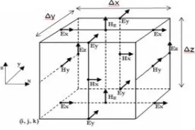
Spatial discretization is achieved by subdividing the computation space in cells called Yee cells (Fig.1). Each cell is marked by indices (i, j, k) and whose space steps
Δx, Δy and Δz are depending on the smaller wavelength in the analysis frequency band of the structure under test.
Figure 1 : Implementation of the Components of the Electric and Magnetic Fields in a Cell Yee
For uniform time discretization, with a sampling step Δt, and an index n that corresponds to the real time n.Δt. In other side components of the electric field and electric flux are calculated for multiple peers of Δt/2, whereas the components of the magnetic field and magnetic flux are calculated for odd multiples of Δt/2.
Thus, the ratings will be used as in the following two examples :
For electric field component ⃒, , . (iΔx, jΔy, kΔz + 0.5Δz; Δt)
For magnetic field component ⃒ . , ,. . (iΔx + 0.5Δx, jΔy, kΔz +
0.5Δz; Δt + 0.5Δt)
2. Rectangular Patch Antenna Study
we proposed to apply the FDTD method to modeling a rectangular patch antenna whose dimensionsare shown in Figure2 [5]. So we are interested to resolving 12 equations concerning field components variation that are evaluated in the following order Dx, Dy, Dz, Ex, Ey, Ez, Bx, By, Bz, Hx, Hy, Hz .
The computational space is composed of two parts, one for the antenna and the second for the conditions UPML which is surrounded by surface type PEC (Perfect Conductor Electric), where the electric field must be zero which allows the updating of the fields in the calculation algorithm.
The stability condition for the algorithm of the FDTD method is given by the inequality (12), [4]
Δ ≤ andΔt ≤ Δ
√ (12)
Or λmin is minimum wave length corresponding to the maximum frequency
supported by thestructure beingstudied and the C0 is the velocity of light in vacuum.
Thus, for three-dimensional (n = 3), we can take Δt = .
For the excitation source in the SP plan (Source Plan), we can choose a Gaussian pulse whose function is given by the expression (13) . It will be added to all components Ez in the FDTD algorithm. With t0=120.Δt andtw=30.Δt in order to
generate a wave in TEM mode.
( ) = exp − (13)
The maximum supported by the studied structure frequency is about 50GHz, spatial and temporal steps discretization adopted for this case will be Δ=0.256 mm et
Δt=O.441 ps .
Where the space problem has the size of 70x16x150 cells. UPML conditions occupies 19 cells for each of six face. Therefore the size of the computing space is 106x186x52 cells .
The modeling algorithm for this antenna uses 30 coefficients existing in 12 equations in order to evaluate electric and magnetic components fields. This requires in total 42 three dimensional matrices, where each matrix is the size 106x186 x 52.
The result of this modeling is the reflection coefficient S11. At Terminal plane (TP), shown in Figure2 and which is located at a distance of 10.Δ for source plane
(SP) level, we estimate de value of the coefficient S11, that the expression in (14), by
revaluing incident and reflected wave given by the components Ez or Hx.
( ) = ( )
( )=
( ) ( )=
( )
( ) = 10log (| |) (15)
To obtain S11(f), we used Fourier transformation witch is given by the
MATLAB (Fast Fourier Transform) function (FFT). Then we evaluated the variation of the reflection coefficient S11(dB), whose expression in (15) as a function of the
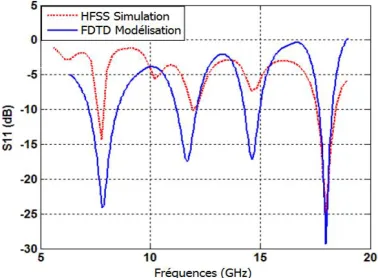
frequency. The graph is shown in Figure 3.On the same Figure also are shown the results of the simulation by the HFSS Soft.
Figure 3. Variation Coefficient S11 Depending on the Frequency for
Rectangular Patch Antenna
It is noted that the two curves have the same shape and magnitude is approached. The slight difference may be explained by the distortion of source witch must be carefully chosen.
By comparing the resonance frequencies from the cavity model, we find that the resonance frequency of the antenna is usable in TM020 mode is given by
:( ) =
√ = 8.1 GHZ.
On the other hand, the input impedance of the patch antenna at terminal plan (TP) is related to the reflection coefficient S11 by expression (18)
= (18)
With Z0 = 50Ω is the characteristic impedance of the feed line.
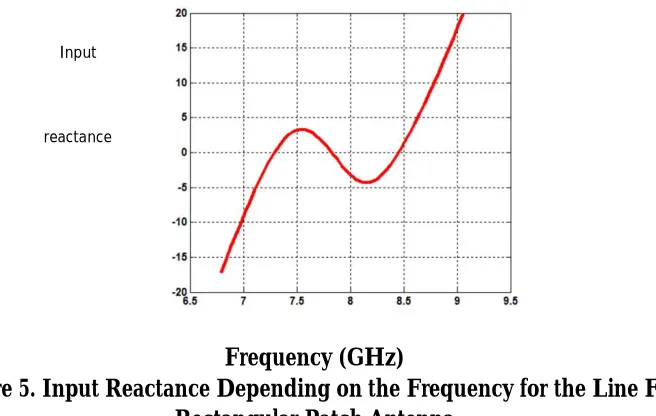
The variation of the resistance and the reactance according to the frequency are shown in Figures 4 and 5.
Frequency (GHz)
Figure 4. Input Resistance Depending on the Frequency for the Line Fed Rectangular Patch Antenna
Frequency (GHz)
Figure 5. Input Reactance Depending on the Frequency for the Line Fed Rectangular Patch Antenna
Input
resistance
Input
The Figure4 shows that at the resonance frequency of 7.8Ghz, Input resistance is approximately 46Ω. This value is close to the characteristic impedance of the feed line which is 50Ω
From Figure 5, it is found that the reactance at the resonant frequency is zero and that is ideal for the resonance. Since the input impedance of the patch antenna in the terminal plane (TP) is known, we can estimate antenna input impedance Zin defined by (19).
= (19)
β (rad/m) is the phase constant of the line fed, phase velocity and effective dielectric constant can be calculated from the expressions (20), (21) and (22).
= (20)
= (21)
= +
⁄ (22)
3. Conclusion
References
Khor, W., Bialkowski, M., Abosh, A., Seman, N., Crozier, S. (2006) .An Ultra Wideband
Microwave ImagingSystem for Breast Cancer Detection.International Symposium on Antennas Propagation, Piscalaway ISAP, 1-5.
Sevgi, L., (2003).Complex Electromagnetic Problems and Numerical Simulation Approaches. Wiley-IEEEPress,ISBN 978-0-471-43062-9, 342-346.
Balanis,C. A. (2005) . Antenna Theory Analysis and design( 3th Edition) . John Wiley & Sons.
Taflove, C. A., Hagness,S. (2005) .Computationnal Electrodynamics: The Finite-Difference Time Domain method (3th Edition) . Artech House .