Real-time relative permeability prediction using deep learning.

deep learning.

Journal of petroleum exploration and production technologies

[online], 9(2), pages 1271-1284.

Available from:

https://doi.org/10.1007/s13202-018-0578-5

Real-time relative permeability prediction using

deep learning.

ARIGBE, O.D., OYENEYIN, M.B., ARANA, I., GHAZI, M.D.

2019

https://doi.org/10.1007/s13202-018-0578-5

ORIGINAL PAPER - PRODUCTION ENGINEERING

Real-time relative permeability prediction using deep learning

Received: 3 May 2018 / Accepted: 2 November 2018 / Published online: 24 November 2018 © The Author(s) 2018

Abstract

A review of the existing two- and three-phase relative permeability correlations shows a lot of pitfalls and restrictions imposed by (a) their assumptions (b) generalization ability and (c) difficulty with updating in real-time for different reservoirs sys-tems. These increase the uncertainty in its prediction which is crucial owing to the fact that relative permeability is useful for predicting future reservoir performance, effective mobility, ultimate recovery, and injectivity among others. Laboratory experiments can be time-consuming, complex, expensive and done with core samples which in some circumstances may be difficult or impossible to obtain. Deep Neural Networks (DNNs) with their special capability to regularize, generalize and update easily with new data has been used to predict oil–water relative permeability. The details have been presented in this paper. In addition to common parameters influencing relative permeability, Baker and Wyllie parameter combinations were used as input to the network after comparing with other models such as Stones, Corey, Parker, Honapour using Corey and Leverett-Lewis experimental data. The DNN automatically used the best cross validation result (in a five-fold cross validation) for its training until convergence by means of Nesterov-accelerated gradient descent which also minimizes the cost function. Predictions of non-wetting and wetting-phase relative permeability gave good match with field data obtained for both validation and test sets. This technique could be integrated into reservoir simulation studies, save cost, optimize the number of laboratory experiments and further demonstrate machine learning as a promising technique for real-time reservoir parameters prediction.

Keywords Deep neural networks · Relative permeability · Training · Validation · Testing Abbreviations

Kro Oil relative permeability

Krw Water relative permeability

Sw Water saturation

Swc Irreducible water saturation

So Oil saturation

cv Cross validation val Validation dataset dnn Deep neural network σ Standard deviation n Number of samples

Introduction

Relative permeability is the most important property of porous media to carry out reservoir prognosis in a mul-tiphase situation (Delshad and Pope 1989; Yuqi and; Dacun

2004) and therefore needs to be as accurate and readily accessible as possible. Theoretically, it is the ratio of effec-tive and absolute permeability. It is useful for the determina-tion of reservoir productivity, effective mobility, wettability, fluid injection for EOR, late-life depressurization, gas con-densate depletion with aquifer influx, injectivity, gas trap-ping, free water surface, residual fluid saturations, temporary gas storage amongst others (Fig. 1). It is well known that a significant variation in relative permeability data can have a huge impact on a macroscopic scale.

The oil and gas industries have a need for easily avail-able and reliavail-able relative permeability data, expense reduction on experiments and a more general model for the parameter judging by the pitfalls pointed out by several researchers (Table 1) after testing the existing two- and three-phase relative permeability models. Such workers O. D. Arigbe

[email protected]

1

School of Engineering, Sir Ian Wood Building, Robert Gordon University, Aberdeen, UK

2 _{School of Computing and Digital Media, Sir Ian Wood}

like Fayers and Matthews (1984) and Juanes et al. (2006), after testing non-wetting relative permeability interpola-tion models such as Baker and Stone’s I and II, against Saraf et al. (1982), Schneider and Owens (1970), Saraf and Fatt (1967) and Corey et al. (1956) experimental data, pre-sented the same conclusion that they give similar results for high oil saturations but are different as it tends towards residual oil saturation. Manjnath and Honarpour (1984) concluded that Corey gives higher values for non-wetting phase relative permeability after comparing against Don-aldson and Dean data.

Based on the assumption that water and gas relative per-meability depends only on their saturation and not on that of other phases, Delshad and Pope (1989) concluded after a comparative study of seven relative permeability mod-els that Baker and Pope performed better but also stated the need for better models. Siddiqui et al. (1999) found Wyllie-Gardner and Honarpour to yield consistently better results at experimental condition after testing ten relative permeability models. Al-Fattah and Al-Naim (2009) found Honarpour regression model to be the best after comparing with five other models and also developed his own regres-sion model. Since the coefficients of these regresregres-sion mod-els are not generalized, they are not suitable for real-time applications.

Furthermore, for wetting phase relative permeability in consolidated media, Li and Horne (2006) showed that the Purcell model best fits the experimental data in the

cases studied by them provided the measured capillary pressure curve had the same residual saturation as the relative permeability curve which is sometimes not the case. Saraf and McCaffery (1985) could not recommend a best model due to scarcity of three-phase relative per-meability data. The different relative perper-meability cor-relations have limitations and assumptions which no doubt have implications, thus increasing the uncertainty in reservoir simulation studies hence the need for a more generalized model.

Therefore, the purpose of this study is to implement a Deep Neural Networks model for the prediction of rela-tive permeability accounting for reservoir depletion, satu-ration and phase changes with time. Guler et al. (1999) developed several neural network models for relative per-meability considering different parameters that affects the property and selected the best model to make predictions for the test set while Al-Fattah (2013) also used a general-ized regression neural network to predict relative permea-bility. Getting better prediction for out-of-sample datasets (better generalization), performance flattening out with a certain amount of data (scalability) as well as requiring far more neurons (and hence an increased computational time) to achieve better results as deep learning models is an issue for such networks. Again most of the reviewed empirical models can hardly generalize (Du Yuqi et al.

2004) and are static but deep neural networks (with its advanced features), if appropriately tuned, can capture the Fig. 1 Schematic of oil–water

transients faster and more accurately throughout the res-ervoir life while also getting better as more data becomes available with time. Training can be done offline and the trained networks are suitable for on-board generation of descent relative permeability profiles as their computa-tion requires a modest CPU effort hence not a concern to real-time application.

Methodology

The most commonly available factors influencing rela-tive permeability such as porosity, ᙃ; viscosity, μ; per-meability k; saturation s, together with Baker and Wyl-lie parameter combinations were used as inputs for the network. Baker gave correlation coefficients of 0.96 and 0.86 while Wyllie has correlation coefficients of 0.91 and 0.89 for Corey and Leverett-Lewis datasets, respectively (Table 2). There were a total of 12 input parameters fed into the network as shown in Table 3 after testing the sensitivity of several parameter combinations.

Ten (10) sets of water–oil relative permeability data with 132 data points from a North Sea field with four-fifths used as training set and one-fifth as validation set. Another set of water–oil relative permeability data from a separate field were used as the testing set after data wran-gling and normalization. A seed value was set to ensure the repeatability of the model. An optimised number of hidden layers was used to reduce the need for feature engineering. The best cross validation result in a fivefold arrangement was automatically used to train the DNN models until convergence using Nesterov-accelerated gra-dient descent (which minimize their cost function). The Rectifier Linear Units (ReLUs) were used in the DNN modelling to increase the nonlinearity of the model, sig-nificantly reduce the difficulty in learning, improve accu-racy and can accept noise (Eq. 1). This allows for effec-tive training of the network on large and complex datasets making it helpful for real-time applications compared to the commonly used sigmoid function which is difficult to train at some point.

where Y∼ℵ(0,𝜎(x)) is the Gaussian noise applied to the ReLUs.

Separate models were constructed for wetting and non-wetting phases as they have also been found to improve predictions (Guler et al. 1999). They were then validated and tested to check the generalization and stability of the models for out-of-training sample applications.

The developed Deep Neural Networks model could fur-ther be applied to predict ofur-ther experimental data carried

(1)

f(x) =max(0, x+Y),

out based on Buckley and Leverett (1942) frontal advance theory (Fig. 2) and Welge (1952) method for average water saturation behind the water front using the saturation his-tory to make predictions of relative permeability as a func-tion of time.

Deep neural networks

Deep neural networks (sometimes referred to as stacked neural network) is a feed-forward, artificial neural network with several layers of hidden units between its inputs and outputs. One hundred hidden layers with twelve neurons each (100, 12) were used in this work. The ability of the model to transfer to a new context and not over-fit to a specific context (generalization) was addressed using cross validation which is described in detail below. All networks were trained until convergence with Nesterov-accelerated gradient descent which also minimizes the cost function. In addition, both 𝜆1 and 𝜆2 regularization (Eq. 2) were used to add stability and improve the generalization of the model. This regularization ability was further improved by implementing dropout. A copy of the global models parameters on its local data is trained at each computed node with multi-threading asynchronously and periodi-cally contributes to the global model through averaging across the network.

Mathematically,

where x are inputs, 𝜃 are parameters, 𝝀 is a measure of com-plexity by introducing a penalty for complicated and large parameters represented as l1 or l2 (preferred to l0 for con-vexity reasons). They are well suited for modelling systems with complex relationships between input and output which is what is obtainable in natural earth systems. In such cases with no prior knowledge of the nature of non-linearity, tra-ditional regression analysis is not adequate (Gardner and Dorling 1998). It has been successfully applied to real-time speech recognition, computer vision, optimal space craft landing etc.

Cross validation

Overfitting which is the single major problem of pre-diction when independent datasets is used was reduced through cross validation by estimating out-of-sample error rate for the predictive functions built to ensure gen-eralization. Other issues like variable selection, choice of prediction function and parameters and comparison of (2) J(𝜃) = 1 2 n ∑ i=1 ( 𝜃T_x(i)_−y(i))2_+𝜆∑p j=1 𝜃2 j,

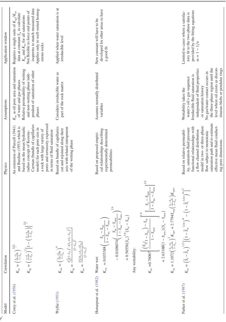
Table 1

Assumptions and application of t

he commonl y used tw o- and t h ree-phase relativ e per meability cor relations Model Cor relation Ph y sics Assumptions Application windo w Core y e t al. ( 1956 ) Kro = ( So − Sor 1 − Sor ) 2 + 3 𝜆 𝜆 Krg = ( 1− So 1 − Sor )2 [ 1− ( So − Sor 1 − Sor )] 2 + 𝜆 _𝜆 An e xtension of Purcell (1941)

and Burdine (1953) whic

h is based on t he mean h ydraulic radius concept of K ozen y -Car

man (bundle of capillar

ies model) f or eac h pore size in a r o ck wit h lar g e v ar ie ty of

pores and tor

tuosity e xpressed in ter ms of fluid saturation Kro ∝

oil pore area and saturation

of w ater and g as phases R elativ e per meability of w etting and non-w

etting phase

inde-pendent of saturation of o

ther

phases

R

eq

uires a single suite of

Krg ∕ Kro dat a at cons tant Sw to calculate Krg and Kro f or all saturations N o t fle xible to f o

rce end points of

isoper ms to matc h measured dat a Applies onl y to w ell-sor ted homog-enous r o ck s W y llie ( 1951 ) Krw = ( Sw − Swc 1 − Swc )4 Krg = S 2 g [ 1( − S)wc 2−( Sw + So − S)wc 2 ] ( 1 − S)wc 4 Kro = S 3 o2( Sw + So − 2 S)wc ( 1 − S)wc 4

Based on bundle of capillar

ies

cut and rejoined along t

heir axis wit h related entrapment of t he w etting phase Considers ir reducible w ater as par t of t he r o ck matr ix Applied when w ater saturation is at ir reducible le v el Honar pour e t al. ( 1982 ) W ater w et: Krw = 0.035388 ( Sw − Swc 1 − Swc − Sorw ) − 0.0108074 ( Sw − Sorw 1 − Swc − Sorw )2.9 + 0.56556 ( Sw )3.6 ( Sw − Swc ) An y w ett ability : Kro = 0.76067 ⎡ ⎢ ⎢ ⎢ ⎣ (/ So 1 − Swc ) − Sor 1 − Sorw ⎤ ⎥ ⎥ ⎥ ⎦ 1.8 [ So − Sorw 1 − Swc − Sorw ]2.0 + 2.6318 ∅ ( 1− Sorw )( S o − Sorw ) Krg = 1.1072 ( Sg − Sgr 1 − Swc )2 K rg o + 2.7794 Sorg ( Sg − Sgr 1 − Swc ) K rgro Based on pr oposed empir

i-cal relationships descr

ibing exper iment all y de ter mined per meabilities Assumes nor mall y dis tr ibuted v ar iables N ew cons tant will ha v e to be de v eloped f or o ther areas to ha v e a good fit P ar k er e t al. ( 1987 ) Kro = ( St − Sw )1∕ 2 [( 1 − Sw 1 ∕ m )m − ( 1− St 1 ∕ m )m ]2 Based on relativ e per meabil-ity , saturation-fluid pressure

functional relationships wit

h a flo w c hannel dis tr ibution model in tw o- or t h ree-phase flo w subject to mono tonic saturation pat h and to es timate effectiv

e mean fluid

conduct-ing pore dimensions

W ett ability t ak es t he w ater > oil > g as seq uence Ir

reducible fluid saturation is independent of fluid pr

oper ties or saturation his tor y N o g as/w ater cont act occurs in the t h

ree-phase region until t

he le v el where oil e xis ts as

discon-tinuous blobs or pendular r

ings

Limited to cases where a satisf

ac-tor y fit to t he tw o-phase dat a is pr o vided b y t he fitting eq uations m = 1 − 1 ∕ n

different predictors were also addressed. A fivefold cross validation technique was used to split the data set into training and test set, build a model on the training set, evaluate on the test set and then repeat and average the errors estimated. A weight decay was chosen to improve the generalization of the model by suppressing any irrel-evant component of the weight vector while solving the learning problem with the smallest vector. This also sup-presses some of the effects of static noise on the target if chosen correctly and increases the level of confidence in the prediction (Fig. 3).

Results and discussion

Deep neural networks model has been validated using separate out-of-sample datasets not used for the train-ing. The good agreement between experimental data and DNN’s model predictions indicates that the complex, transient, non-linear behaviour of reservoir fluids can be effectively modelled as their saturation and phase changes with time.

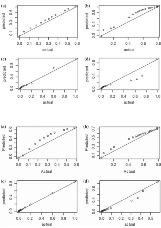
Figures 4, 5 and 6 give a comparison between actual experimental values and model predictions using neural networks without cross validation, neural networks with cross validation and the deep neural networks. The objec-tive here was to see how deep learning out performs ordi-nary networks on new data. These cross plots show the extent of agreement between the laboratory and predicted values. For the testing set drawn from a different field from the training set, the deep neural networks for both the wetting and non-wetting phase relative permeability (Fig. 6b and d) gives very close values to the perfect cor-relation line in all data points compared to the other mod-els. Figure 4a and c representing neural networks without cross validation, gave an RMS value of 0.2484 and 0.0767 while neural net with cross validation gave an RMS of 0.0624 and 0.0765 (Fig. 5a and c). The deep neural net gave an RMS value of 0.2517 and 0.065 (Fig. 6a and c) for both wetting and non-wetting relative permeability. It is clear that all the models did well for the validation set although the deep neural networks performed better than the other two models. The different models were then shown new data from a separate field to see how they performed. For the test set (which is an out-of-sample dataset) obtained from a different field, the RMS for neu-ral network without cross validation is 0.9996 and 0.8483 (Fig. 4b and d), 0.2295 and 0.8022 with cross validation (Fig. 5b and d) while DNNs gave 0.0759 and 0.15 (Fig. 6b and d) for wetting and non-wetting relative permeability, respectively.

The deep learning model used the fourth cross validation model which happen to be the best for the

Table 1 (continued) Model Cor relation Ph y sics Assumptions Application windo w Bak er ( 1988 ) Kro = ( Sw − S)wc Krow +( Sg − S)gr Kro g ( Sw − S)wc +( Sg − S)gr Krw = ( So − S)or Krw o +( Sg − S)gr Krw g ( So − S)or +( Sg − S)gr Krg = ( So − S)or Krg o +( Sw − S)wc Krg w ( So − S)or +( Sw − S)wc As t he saturation of a phase tends to zer o, t hat of t he o ther tw

o-phase will dominate

The end points of t

he t h ree-phase relativ e per meability isoper ms coincide wit h t he tw o-phase relativ e per meability dat a W eighting f actors ( Sw − Swc ) and ( Sg − Sgr ) mus t be bo th positiv e Lomeland e t al. ( 2005 ) Krow = K x ro ( 1 − S)wn L w o ( 1 − S)wn L w o+ E w oS Tw o wn Krw = K o rw Swn L o w Swn L o w+ E o wS T o w wn Swn = Sw − Swi 1 − Swi − Sorw Based on t he mean h ydraulic radius concept of K ozen y -Car

man (bundle of capillar

ies model) Assumes t hat t he whole spec-tr um of t he relativ e per meabil-ity cur v

e can be captured wit

h the L , E , T parame ters It e

xhibits enough fle

xibility to reconcile t he entire spectr um of exper iment al dat a

Table 2 Comparison of relative permeability models (vertical) with different datasets (horizontal) using correlation coefficient (Modified after Baker 1988)

Data Corey Leverett and Lewis

Reid Snell Saraf et al Hosain Guckert

Stone I 0.97 0.76 0.90 0.57 0.82 0.85 0.48

Stone II 0.77 0.75 0.87 0.75 0.68 0.33 0.50

Aziz and Setarri 0.8 0.75 0.95 0.75 0.74 0.9 0.48

Corey 0.88 0.83 0.89 0.48 0.50 0.74 0.6

Baker 0.96 0.86 0.88 0.58 0.9 0.84 0.57

Naar and Wygal 0.74 0.67 0.78 0.50 0.55 0.54 0.50

Parker 0.85 0.73 0.88 0.56 0.87 0.93 0.52

Land 0.93 0.8 0.89 0.50 0.66 0.74 0.55

Wyllie 0.91 0.89 – – – – –

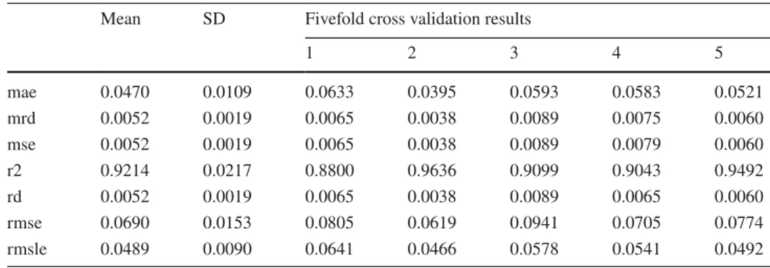
Table 3 Accuracy of the Deep Learning model for the wetting phase with cross validation for the five folds

Mean SD Fivefold cross validation results

1 2 3 4 5 mae 0.0489 0.0068 0.0558 0.0477 0.0612 0.0330 0.0468 mrd 0.0052 0.0022 0.0053 0.0047 0.0108 0.0014 0.0038 mse 0.0052 0.0022 0.0053 0.0047 0.0108 0.0014 0.0038 r2 0.9259 0.0186 0.9121 0.9086 0.9018 0.9745 0.9325 rd 0.0052 0.0022 0.0053 0.0047 0.0108 0.0014 0.0038 rmse 0.0689 0.0150 0.0728 0.0684 0.1037 0.0380 0.0615 rmsle 0.0541 0.0130 0.0509 0.0558 0.0854 0.0277 0.0509

Fig. 2 Water fractional flow curve with its derivative for the field considered 0 0.5 1 1.5 2 2.5 3 3.5 0 0.1 0.2 0.3 0.4 0.5 0.6 0.7 0.8 0.9 1 0 0.2 0.4 0.6 0.8 1 Derivave, dfw/dSw Water Fraconal Flow. Fw Water Saturaon frac flow dfw/dsw

wetting phase with a correlation coefficient of about 97% (Table 3) and the lowest training error of 0.0014 while the second cross validation model was used for the non-wetting phase relative permeability having 96% correla-tion coefficient and the lowest training error value of 0.030 (Table 4).

Figures 7 and 8 display the trend comparing the different models using the standard relationship between saturation and relative permeability. The deep learning model clearly out performs the other models giving better predictions for both the wetting and non-wetting phases. Measurement error which causes input values to differ if the same example is presented to the network more than once is evident in the data. This limits the accuracy of generalization irrespective of the volume of the training set. The deep neural networks model deeply understands the fundamental pattern of the data thus able to give reasonable predictions than ordinary

networks and empirical models (Figs. 9, 10). The curves show that significant changes in the saturation of other phases has large effect on the wetting phase ability to flow as observed from the less flattening of the water relative permeability curve and vice versa for the flattened curve. Although this flattening behaviour is usual in the secondary drainage and imbibition cycles but mainly in the wetting phase when flow is mainly through small pore networks. Again, the curve flattening of the oil relative permeability curve could from experience be from brine sensitivity and high rates causing particle movements resulting in forma-tion damage.

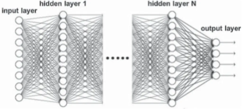
Figures 9 and 10 compares the deep neural network model with commonly used empirical relative permeabil-ity models like Baker, Wyllie, Honarpour, Stones, Corey, Parker. Despite the fact that some of these models were developed using lots of datasets way more than the amount Fig. 3 Deep neural network

model architecture showing input, hidden and output layers (Lee et al. 2017)

Fig. 4 Actual vs predicted value for neural networks without cross validation (cross valida-tion not considered as part of the model formulation) with a

wetting phase relative perme-ability for validation set, b

wetting phase relative perme-ability for test set, c non-wetting relative permeability for valida-tion set, d non-wetting relative permeability for the test set

used for training the deep neural networks, it still out per-formed them showing that it is more able to capture the transients and eddies in real-time scenarios due to its ability to regularize and generalize using its robust parameters as discussed earlier.

Figures 11 and 12 corroborate the earlier observation that the deep learning model predicts better compared to most of the relative permeability models used in reservoir modelling software. It is important to note here that the empirical mod-els (Figs. 9, 10) have a problem of generalization especially

as every reservoir is unique. Again, the assumptions associ-ated with their formulation might not be practically true in all cases but this reservoir uniqueness or generalization is captured by the deep learning model bearing in mind that it will perform even better as more real-time data are added to the training set.

Figures 13 and 14 describe the relative importance (sensi-tivity) of the variables used for the wetting and non-wetting deep learning relative permeability models. The wetting phase model was more sensitive to its saturation and relatively less Fig. 5 Actual vs predicted

value for neural networks with cross validation technique used for its model formulation and it improved prediction ability of the network with a wetting phase relative permeability for validation set, b wetting phase relative permeability for test set,

c non-wetting relative perme-ability for validation set, d non-wetting relative permeability for the test set

Fig. 6 Actual vs predicted value for deep neural networks model with a wetting phase relative permeability for validation set,

b wetting phase relative perme-ability for test set, c non-wetting relative permeability for valida-tion set, d non-wetting relative permeability for the test set

sensitive to that of the non-wetting phase while the non-wet-ting phase model was very sensitive to both its saturation and that of the wetting phase. Both models were also more sen-sitive to their own viscosities than the other. These models seem to obey the basic physics underlying relative permeabil-ity modelling. The least important variable still contributed above the median mark although in general, all variables show greater sensitivity in the non-wetting model than in the wetting relative permeability model. Table 5 shows the performance of the different variables combinations for both the wetting and non-wetting phase model.

Conclusion

A deep neural network methodology has been formulated for wetting and non-wetting phase relative permeabil-ity predictions taking into account phase and saturation

changes hence its capability for real-time applications. This work has the following conclusions:

1. Deep neural network has shown to be a good predictive and prescriptive tool for relative permeability than ordi-nary networks. Its ability to generalize and regularize helped to stabilize and reduce the main problem of all predictive tools which is over fitting.

2. Different results were obtained from different relative permeability models for the same reservoir with some of the models giving better predictions at lower satura-tions but performs poorly at higher saturasatura-tions and vice versa; hence, lots of uncertainty. Therefore, it is needful for practitioners to know the limitations of any correla-tion used for the prediccorrela-tion of wetting and non-wetting phase relative permeability.

3. In an industry where big data is now available, deep learning can provide the platform to systematically Table 4 Accuracy of the

deep learning model for the non-wetting phase with cross validation for the fivefolds

Mean SD Fivefold cross validation results

1 2 3 4 5 mae 0.0470 0.0109 0.0633 0.0395 0.0593 0.0583 0.0521 mrd 0.0052 0.0019 0.0065 0.0038 0.0089 0.0075 0.0060 mse 0.0052 0.0019 0.0065 0.0038 0.0089 0.0079 0.0060 r2 0.9214 0.0217 0.8800 0.9636 0.9099 0.9043 0.9492 rd 0.0052 0.0019 0.0065 0.0038 0.0089 0.0065 0.0060 rmse 0.0690 0.0153 0.0805 0.0619 0.0941 0.0705 0.0774 rmsle 0.0489 0.0090 0.0641 0.0466 0.0578 0.0541 0.0492

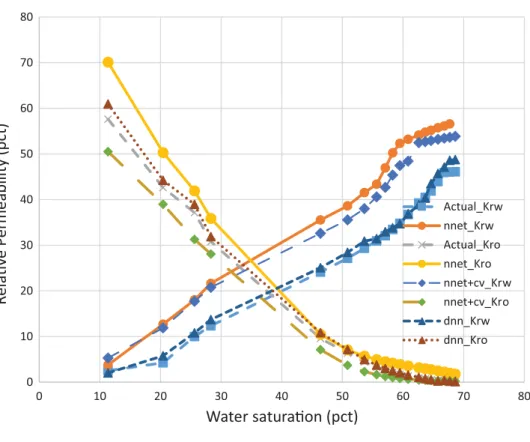
Fig. 7 Experimental and predicted relative permeability models using neural network with and without cross valida-tion and deep neural networks on the validation set. The neural network model with cross validation (cv) partitioned the dataset into fivefold and then trained and tested the model using the different folds

0 10 20 30 40 50 60 70 80 90 100 0 10 20 30 40 50 60 70 80

R

elav

e P

ermeability

(pct)

Water saturaon (pct)

Fig. 8 Experimental (actual) and predicted relative perme-ability models using neural network (both with and without cross validation) and deep neural networks on the out-of-sample test set (Stafjord reservoir). Cross validation (cv) involved in the network helped to improve its accuracy for out-of-sample datasets 0 10 20 30 40 50 60 70 80 0 10 20 30 40 50 60 70 80

R

elav

e P

ermeability

(pct)

Water saturaon (pct)

Fig. 9 Comparison of Wyllie, Corey, Parker, Stone, Baker, Honarpour, deep neural net-works for the Brent reservoir, North Sea. The DNN gave bet-ter prediction than the existing models for this validation set. Corey’s,𝜆, taken to be 2 and Parker’s n parameter

0.01 0.1 1 10

dnn Hon Baker Wyllie Corey Stone 1 Parker

rmse

models

kro_test kro_validaon

Fig. 10 Comparison of Wyllie, Corey, Baker, Honarpour, deep neural networks models for the Stratjford reservoir, NorthSea

0.01 0.1 1 10

dnn Hon Baker Wyllie Corey

rmse

models

krw_test krw_validaon

Fig. 11 Comparison of deep neural networks and Baker with the measured wetting and non-wetting relative permeability models for the validation set (Brent reservoir) 0 10 20 30 40 50 60 70 80 90 100 0 10 20 30 40 50 60 70 80 Relave Permeability (pct) Water saturaon (pct) actual_Kro actual__Krw dnn_krw dnn_kro kro_baker krw_baker

forecast reservoir fluid and rock properties to drastically optimize the cost and time needed for laboratory experi-ments. Even with the amount of data used, the power

of the deep neural networks is evident in that it gave reasonable predictions which will dramatically improve if more data were available.

Fig. 12 Comparison of deep neural networks and Baker with the wetting and non-wetting phase relative permeability models with for the test sets (Stratjford reservoir). Baker was used since it performed best among the models compared

0 10 20 30 40 50 60 70 80 90 100 0 10 20 30 40 50 60 70 80 Relave Permeability (pct) Water saturaon (pct) actual_Kro actual__Krw dnn_kro dnn_krw krw_baker kro_baker

Fig. 13 Sensitivity analysis of individual variables used for building the wetting phase deep learning relative permeability model 0 0.2 0.4 0.6 0.8 1 Sw-Swi Sw Uw 1-Swi So Uo Phi Sor So-Sor Swi Uo/Uw K Relave Importance Variables

Open Access This article is distributed under the terms of the Crea-tive Commons Attribution 4.0 International License (http://creat iveco

mmons .org/licen ses/by/4.0/), which permits unrestricted use,

distribu-tion, and reproduction in any medium, provided you give appropriate credit to the original author(s) and the source, provide a link to the Creative Commons license, and indicate if changes were made.

References

Al-Fattah SMA (2013) Artificial neural network models for determin-ing relative permeability of hydrocarbon reservoirs. U.S. Patent No. 8,510,242. U.S. Patent and Trademark Office, Washington, DC

Al-Fattah SM, Al-Naim HA (2009) Artificial-intelligence technology predicts relative permeability of giant carbonate reservoirs. SPE Reserv Eval Eng 12(01):96–103

Baker L (1988) Three-phase relative permeability correlations. In: SPE enhanced oil recovery symposium. Society of petroleum engineers Buckley SE, Leverett M (1942) Mechanism of fluid displacement in

sands. Trans AIME 146(01):107–116

Corey A et al (1956) Three-phase relative permeability. J Petrol Tech-nol 8(11):63–65

Delshad M, Pope GA (1989) Comparison of the three-phase oil relative permeability models. Transp Porous Media 4(1):59–83

Du Yuqi OB, Dacun L (2004) Literature review on methods to obtain relative permeability data. In: 5th conference & exposition on petroleum geophysics, Hyderabad, India, pp 597–604

Fayers F, Matthews J (1984) Evaluation of normalized Stone’s methods for estimating three-phase relative permeabilities. Soc Petrol Eng J 24(02):224–232

Gardner MW, Dorling S (1998) Artificial neural networks (the mul-tilayer perceptron)—a review of applications in the atmospheric sciences. Atmos Environ 32(14):2627–2636

Fig. 14 Sensitivity analysis of individual variable used for building the non-wetting phase deep learning relative perme-ability model 0 0.2 0.4 0.6 0.8 1 Sw-Swi So Sw Uo So-Sor Phi Uw Swi K 1-Swi Sor Uo/Uw Relave Importance Variables

Table 5 Sensitivity analysis showing the importance of the difference to both water and oil relative permeabilities

Cases Input parameters Functional links (from Baker and Wyllie) Model metric (RMSE, fraction) Krw Kro 1 S_w, S_o 0.1204 0.1532 2 S_w, S_o, S_wi 0.1201 0.1057 3 S_w, S_o, S_wi,S_or 0.1153 0.0712 4 S_w, S_o, S_wi,S_or,k 0.0906 0.0698

5 Sw, So, Swi,Sor,k, phi 0.0705 0.0671

6 S_w,S_o,S_wi, S_or, k, phi,𝜇_o 0.0616 0.0691 7 S_w,S_o, S_wi,S_or,k, phi,𝜇_o,𝜇_w 0.0481 0.0681 8 S_w, S_o, S_wi,S_or,k, phi,𝜇_o,𝜇_w (_Sw−Swc) 0.0463 0.0667 9 S_w,S_o, S_wi,S_or,k, phi, 𝜇_o, 𝜇_w (_Sw−Swc)_, (_So−Sor) 0.0449 0.0652 10 S_w, S_o, S_wi, S_or, k, phi, 𝜇_o, 𝜇_w (_Sw−Swc)_, (_So−Sor)_, (_1−Swc) 0.0508 0.0732 11 S_w, S_o, S_wi, S_or, k, phi, 𝜇_o, 𝜇_w (_Sw−Swc)_, (_So−Sor)_, (_1−Swc)_, (_{𝜇o∕𝜇w}) 0.0380 0.0619

Guler B, Ertekin T, Grader AS (1999) An artificial neural network based relative permeability predictor. Pet Soc Canada. https ://doi. org/10.2118/99-91

Honarpour M, Koederitz L, Harvey AH (1982) Empirical equations for estimating two-phase relative permeability in consolidated rock. J Pet Technol 34(12):2905–2908

Juanes R et al (2006) Impact of relative permeability hysteresis on geological CO2 storage. Water Resour Res 42:12

Lee B, Min S, Yoon S (2017) Deep learning in bioinformatics. Brief Bioinform 18(5):851–869

Li K, Horne RN (2006) Comparison of methods to calculate relative permeability from capillary pressure in consolidated water-wet porous media. Water Resour Res 42(6):39–48

Lomeland F, Ebeltoft E, Thomas WH (2005) A new versatile rela-tive permeability correlation. In: International Symposium of the Society of Core Analysts, Toronto, Canada, pp 1–12

Manjnath A, Honarpour M (1984) An investigation of three-phase relative permeability. SPE Rocky Mountain Regional Meeting. Society of Petroleum Engineers

Parker JC, Lenhard RJ, Kuppusamy T (1987) A parametric model for constitutive properties governing multiphase flow in porous media. Water Resour Res 23(4):618–624

Saraf D, Fatt I (1967) Three-phase relative permeability measurement using a nuclear magnetic resonance technique for estimating fluid saturation. Soc Petrol Eng J 7(03):235–242

Saraf D, Mccaffery F (1985) Relative permeabilities. Dev Pet Sci 17:75–118

Saraf DN, Batycky JP, Jackson CH, Fisher DB (1982) An experimen-tal investigation of three-phase flow of water-oil-gas mixtures through water-wet sandstones. In: SPE California Regional Meet-ing. Society of Petroleum Engineers

Schneider F, Owens W (1970) Sandstone and carbonate two-and three-phase relative permeability characteristics. Soc Petrol Eng J 10(01):75–84

Siddiqui S, Hicks PJ, Ertekin T (1999) Two-phase relative permeabil-ity models in reservoir engineering calculations. Energy Source 21(1–2):145–162

Welge HJ (1952) A simplified method for computing oil recovery by gas or water drive. J Petrol Technol 4(04):91–98

Wyllie M (1951) A note on the interrelationship between wetting and non-wetting phase relative permeability. J Petrol Technol 3(10):17–17

Publisher’s Note Springer Nature remains neutral with regard to jurisdictional claims in published maps and institutional affiliations.