Bioinformatics Programming Using Python.pdf

(1)

(2)

(3)

(4)

(5)

Bioinformatics Programming

Using Python

Mitchell L Model

(6)

Bioinformatics Programming Using Python by Mitchell L Model

Published by O’Reilly Media, Inc., 1005 Gravenstein Highway North, Sebastopol, CA 95472.

O’Reilly books may be purchased for educational, business, or sales promotional use. Online editions are also available for most titles (http://my.safaribooksonline.com). For more information, contact our corporate/institutional sales department: 800-998-9938 or [email protected].

Editor: Mike Loukides

Production Editor: Sarah Schneider Copyeditor: Rachel Head

Proofreader: Sada Preisch

Indexer: Lucie Haskins

Cover Designer: Karen Montgomery Interior Designer: David Futato Illustrator: Robert Romano

Printing History:

December 2009: First Edition.

O’Reilly and the O’Reilly logo are registered trademarks of O’Reilly Media, Inc. Bioinformatics Pro-gramming Using Python, the image of a brown rat, and related trade dress are trademarks of O’Reilly Media, Inc.

Many of the designations used by manufacturers and sellers to distinguish their products are claimed as trademarks. Where those designations appear in this book, and O’Reilly Media, Inc. was aware of a trademark claim, the designations have been printed in caps or initial caps.

While every precaution has been taken in the preparation of this book, the publisher and author assume no responsibility for errors or omissions, or for damages resulting from the use of the information con-tained herein.

TM

This book uses RepKover, a durable and flexible lay-flat binding.

ISBN: 978-0-596-15450-9

(7)

3. Collections . . . 47

Sets 48

Sequences 51

Strings, Bytes, and Bytearrays 53

Ranges 60

Tuples 61

Lists 62

Mappings 66

Dictionaries 67

Streams 72

Files 73

Generators 78

Collection-Related Expression Features 79

Comprehensions 79

Functional Parameters 89

Tips 94

Traps 96

Tracebacks 97

4. Control Statements . . . 99

Conditionals 101

Loops 104

Simple Loop Examples 105

Initialization of Loop Values 106

Looping Forever 107

Loops with Guard Conditions 109

Iterations 111

Iteration Statements 111

Kinds of Iterations 113

Exception Handlers 134

Python Errors 136

Exception Handling Statements 138

Raising Exceptions 141

Extended Examples 143

Extracting Information from an HTML File 143

The Grand Unified Bioinformatics File Parser 146

Parsing GenBank Files 148

Translating RNA Sequences 151

(9)

Tips 160

Traps 162

Tracebacks 163

5. Classes . . . 165

Defining Classes 166

Instance Attributes 168

Class Attributes 179

Class and Method Relationships 186

Decomposition 186

Inheritance 194

Tips 205

Traps 207

Tracebacks 208

6. Utilities . . . 209

System Environment 209

Dates and Times: datetime 209

System Information 212

Command-Line Utilities 217

Communications 223

The Filesystem 226

Operating System Interface: os 226

Manipulating Paths: os.path 229

Filename Expansion: fnmatch and glob 232

Shell Utilities: shutil 234

Comparing Files and Directories 235

Working with Text 238

Formatting Blocks of Text: textwrap 238

String Utilities: string 240

Comma- and Tab-Separated Formats: csv 241

String-Based Reading and Writing: io 242

Persistent Storage 243

Persistent Text: dbm 243

Persistent Objects: pickle 247

Keyed Persistent Object Storage: shelve 248

Debugging Tools 249

Tips 253

Traps 254

Tracebacks 255

(10)

7. Pattern Matching . . . 257

Fundamental Syntax 258

Fixed-Length Matching 259

Variable-Length Matching 262

Greedy Versus Nongreedy Matching 263

Grouping and Disjunction 264

The Actions of the re Module 265

Functions 265

Flags 266

Methods 268

Results of re Functions and Methods 269

Match Object Fields 269

Match Object Methods 269

Putting It All Together: Examples 270

Some Quick Examples 270

Extracting Descriptions from Sequence Files 272

Extracting Entries From Sequence Files 274

Tips 283

Traps 284

Tracebacks 285

8. Structured Text . . . 287

HTML 287

Simple HTML Processing 289

Structured HTML Processing 297

XML 300

The Nature of XML 300

An XML File for a Complete Genome 302

The ElementTree Module 303

Event-Based Processing 310

expat 317

Tips 322

Traps 323

Tracebacks 323

9. Web Programming . . . 325

Manipulating URLs: urllib.parse 325

Disassembling URLs 326

Assembling URLs 327

Opening Web Pages: webbrowser 328

(11)

Constructing and Submitting Queries 329

Constructing and Viewing an HTML Page 330

Web Clients 331

Making the URLs in a Response Absolute 332

Constructing an HTML Page of Extracted Links 333

Downloading a Web Page’s Linked Files 334

Web Servers 337

Sockets and Servers 337

CGI 343

Simple Web Applications 348

Tips 355

Traps 357

Tracebacks 358

10. Relational Databases . . . 359

Representation in Relational Databases 360

Database Tables 360

A Restriction Enzyme Database 365

Using Relational Data 370

SQL Basics 371

SQL Queries 380

Querying the Database from a Web Page 392

Tips 395

Traps 398

Tracebacks 398

11. Structured Graphics . . . 399

Introduction to Graphics Programming 399

Concepts 400

GUI Toolkits 404

Structured Graphics with tkinter 406

tkinter Fundamentals 406

Examples 411

Structured Graphics with SVG 431

SVG File Contents 432

Examples 436

Tips 444

Traps 445

Tracebacks 447

(12)

A. Python Language Summary . . . 449

B. Collection Type Summary . . . 459

(13)

Preface

This preface provides information I expect will be important for someone reading and using this book. The first part introduces the book itself. The second talks about Python. The third part contains other notes of various kinds.

Introduction

I would like to begin with some comments about this book, the field of bioinformatics, and the kinds of people I think will find it useful.

About This Book

The purpose of this book is to show the reader how to use the Python programming language to facilitate and automate the wide variety of data manipulation tasks en-countered in life science research and development. It is designed to be accessible to readers with a range of interests and backgrounds, both scientific and technical. It emphasizes practical programming, using meaningful examples of useful code. In ad-dition to meeting the needs of individual readers, it can also be used as a textbook for a one-semester upper-level undergraduate or graduate-level course.

The book differs from traditional introductory programming texts in a variety of ways. It does not attempt to detail every possible variation of the mechanisms it describes, emphasizing instead the most frequently used. It offers an introduction to Python pro-gramming that is more rapid and in some ways more superficial than what would be found in a text devoted solely to Python or introductory programming. At the same time, it includes some advanced features, techniques, and topics that are often omitted from entry-level Python books. These are included because of their wide applicability in bioinformatics programming, and they are used extensively in the book’s examples. Python’s installation includes a large selection of optional components called “modules.” Python books usually cover a small selection of the most generally useful modules, and perhaps some others in less detail. Having bioinformatics programming as this book’s target had some interesting effects on the choice of which modules to discuss, and at what depth. The modules (or parts of modules) that are

(14)

covered in this book are the ones that are most likely to be particularly valuable in bioinformatics programming. In some cases the discussions are more substantial than would be found in a generic Python book, and many of the modules covered here appear in few other books. Chapter 6, in particular, describes a large number of narrowly focused “utility” modules.

The remaining chapters focus on particular areas of programming technology: pattern matching, processing structured text (HTML and XML), web programming (opening web pages, programming HTTP requests, interacting with web servers, etc.), relational databases (SQL), and structured graphics (Tk and SVG). They each introduce one or two modules that are essential for working with these technologies, but the chapters have a much larger scope than simply describing those modules.

Unlike many technical books, this one really should be read linearly. Even in the later chapters, which deal extensively with particular kinds of programming work, examples will often use material from an earlier chapter. In most places the text says that and provides cross-references to earlier examples, so you’ll at least know when you’ve en-countered something that depends on earlier material. If you do jump from one place to another, these will provide a path back to what you’ve missed.

Each chapter ends with a special “Tips, Traps, and Tracebacks” section. The tips pro-vide guidance for applying the concepts, mechanisms, and techniques discussed in the chapter. In earlier chapters, many of the tips also provide advice and recommendations for learning Python, using development tools, and organizing programs. The traps are details, warnings, and clarifications regarding common sources of confusion or error for Python programmers (especially new ones). You’ll soon learn what a traceback is; for now it is enough to say that they are error messages likely to be encountered when writing code based on the chapter’s material.

About Bioinformatics

Any title with the word “bioinformatics” in it is intrinsically ambiguous. There are (at least) three quite different kinds of activities that fall within this term’s wide scope. Both the nature of the work performed and the educational backgrounds and technical talents of the people who perform these various activities differ significantly. The three main areas of bioinformatics are:

Computational biology

Concerned with the development of algorithms for mining biological data and modeling biological phenomena

Software development

(15)

Life science research and development

Focused on the application of the tools and results provided by the other two areas to probe the processes of life

This book is designed to teach you bioinformatics software development. There is no computational biology here: no statistics, formulas, equations—not even explanations of the algorithms that underlie commonly used informatics software. The book’s ex-amples are all based on the kind of data life science researchers work with and what they do with it.

The book focuses on practical data management and manipulation tasks. The term “data” has a wide scope here, including not only the contents of databases but also the contents of text files, web pages, and other information sources. Examples focus on genomics, an area that, relative to others, is more mature and easier to introduce to people new to the scientific content of bioinformatics, as well as dealing with data that is more amenable to representation and manipulation in software. Also, and not inci-dentally, it is the part of bioinformatics with which the author is most familiar.

About the Reader

This book assumes no prior programming experience. Its introduction to and use of Python are completely self-contained. Even if you do have some programming experi-ence, the nature of Python and the book’s presentation of technical matter won’t nec-essarily relate directly to anything you’ve learned before: you too might find much to explore here.

The book also assumes no particular knowledge of or experience in bioinformatics or any of the scientific fields to which it relates. It uses real examples from real biological data, and while nearly all of the topics should be familiar to anyone working in the field, there’s nothing conceptually daunting about them. Fundamentally, the goal here is to teach you how to write programs that manipulate data.

This book was written with several audiences in mind: • Life scientists

• Life sciences students, both undergraduate and graduate • Technical staff supporting life science research

• Software developers interested in the use of Python in the life sciences To each of these groups, I offer an introductory message:

Scientists

Presumably you are reading this book because you’ve found yourself doing, or wanting to do, some programming to support your work, but you lack the com-puter science or software engineering background to do it as well as you’d like. The book’s introduction to Python programming is straightforward, and its

(16)

examples are drawn from bioinformatics. You should find the book readable even if you are just curious about programming and don’t plan to do any yourself.

Students

This book could serve as a textbook for a one-semester course in bioinformatics programming or an equivalent independent study effort. If you are majoring in a life science, the technical competence you can gain from this book will enable you to make significant contributions to the projects in which you participate. If you are majoring in computer science or software engineering but are intrigued by bioinformatics, this book will give you an opportunity to apply your technical education in that field. In any case, nothing in the book should be intimidating to any student with a basic background either in one of the life sciences or in computing.

Technical staff

You’re probably already doing some work managing and manipulating data in support of life science research and development, and you may be accustomed to writing small scripts and performing system maintenance tasks. Perhaps you’re frustrated by the limits of your knowledge of computing techniques. Regardless, you have developed an interest in the science and technology of bioinformatics. You want to learn more about those fields and develop your skills in working with biological data. Whatever your training and responsibilities, you should find this book both approachable and helpful.

Programmers

Bioinformatics software differs from most other software in important, though hard to pin down, ways. Python also differs from other programming languages in ways that you will probably find intriguing. This book moves quickly into signifi-cant technical material—it does not follow the pattern of a traditional kind of “Programming in...” or “Learning...” or “Introduction to...” book. Though it makes no attempt to provide a bioinformatics primer, the book includes sufficient examples and explanations to intrigue programmers curious about the field and its unusual software needs.

(17)

Some things that will appear strange to anyone with significant programming experi-ence are in reality true to a pure “Pythonic” approach. It is delightful to have the opportunity to write in this vocabulary without the need to accommodate more tradi-tional terminology.

The most significant example of this is that the word “variable” is never used in the context of assignment statements or function calls. Python does not assign values to variables in the way that traditional “values in a box” languages do. Instead, like some of the languages that influenced its design, what Python does is assign names to values. The assignment statement should be read from left to right as assigning a name to an existing value. This is a very real distinction that goes beyond the ways languages such as Java and C++ refer to objects through pointer-valued variables.

Another aspect of the book’s heavily Pythonic approach is its routine use of compre-hensions. Approached by someone familiar with other languages, these can appear quite mysterious. For someone learning Python as a first language, though, they can be more natural and easier to use than the corresponding combinations of assignments, tests, and loops or iterations.

Python

This section introduces the Python language and gives instructions for installing and running Python on your machine.

Some Context

There are many kinds of programming languages, with different purposes, styles, in-tended uses, etc. Professional programmers often spend large portions of their careers working with a single language, or perhaps a few similar ones. As a result, they are often unaware of the many ways and levels at which programming languages can differ. For educational and professional development purposes, it can be extremely valuable for programmers to encounter languages that are fundamentally different from the ones with which they are familiar.

The effects of such an encounter are similar to learning a foreign human language from a different culture or language family. Learning Portuguese when you know Spanish is not much of a mental stretch. Learning Russian when you are a native English speaker is. Similarly, learning Java is quite easy for experienced C++ programmers, but learning Lisp, Smalltalk, ML, or Perl would be a completely different experience.

Broadly speaking, programming languages embody combinations of four paradigms. Some were designed with the intention of staying within the bounds of just one, or perhaps two. Others mix multiple paradigms, although in these cases one is usually dominant. The paradigms are:

(18)

Procedural

This is the traditional kind of programming language in which computation is described as a series of steps to be executed by the computer, along with a few mechanisms for branching, repetition, and subroutine calling. It dates back to the earliest days of computing and is still a core aspect of most modern languages, including those designed for other paradigms.

Declarative

Declarative programming is based on statements of facts and logical deduction systems that derive further facts from those. The primary embodiment of the logic programming paradigm is Prolog, a language used fairly widely in Artificial Intel-ligence (AI) research and applications starting in the 1980s. As a purely logic-based language, Prolog expresses computation as a series of predicate calculus assertions, in effect creating a puzzle for the system to solve.

Functional

In a purely functional language, all computation is expressed as function calls. In a truly pure language there aren’t even any variable assignments, just function parameters. Lisp was the earliest functional programming language, dating back to 1958. Its name is an acronym for “LISt Processing language,” a reference to the kind of data structure on which it is based.

Lisp became the dominant language of AI in the 1960s and still plays a major role in AI research and applications. The language has evolved substantially from its early beginnings and spawned many implementations and dialects, although most of these disappeared as hardware platforms and operating systems became more standardized in the 1980s.

A huge standardization effort combining ideas from several major dialects and a great many extensions, including a complete object-oriented (see below) compo-nent, was undertaken in the late 1980s. This effort resulted in the now-dominant CommonLisp.*_{Two important dialects with long histories and extensive current}

use are Scheme and Emacs Lisp, the scripting language for the Emacs editor. Other functional programming languages in current use are ML and Haskell.

Object-oriented

Object-oriented programming was invented in the late 1960s, developed in the research community in the 1970s, and incorporated into languages that spread widely into both academic and commercial environments in the 1980s (primarily Smalltalk, Objective-C, and C++). In the 1990s this paradigm became a key part of modern software development approaches. Smalltalk and Lisp continued to be used, C++ became dominant, and Java was introduced. Mac OS X, though built on a Unix-like kernel, uses Objective-C for upper layers of the system, especially the user interface, as do applications built for Mac OS X. JavaScript, used primarily to program web browser actions, is another object-oriented language. Once a

(19)

radical innovation, object-oriented programming is today very much a mainstream paradigm.

Another dimension that distinguishes programming languages is their primary inten-ded use. There have been languages focused on string matching, languages designed for embedded devices, languages meant to be easy to learn, languages built for efficient execution, languages designed for portability, languages that could be used interac-tively, languages based largely on list data structures, and many other kinds.

Language designers, whether consciously or not, make choices in these and other dimensions. Subsequent evolutions of their languages are subject to market forces, intellectual trends, hardware developments, and so on. These influences may help a language mature and reach a wider audience. They may also steer the language in directions somewhat different from those originally intended.

The Python Language

Simply put, Python is a beautiful language. It is effective for everything from teaching new programmers to advanced computer science study, from simple scripts to sophis-ticated advanced applications. It has always had some purchase in bioinformatics, and in recent years its popularity has been increasing rapidly. One goal of this book is to help significantly expand Python’s use for bioinformatics programming.

Python features a syntax in which the ends of statements are marked only by the end of a line, and statements that form part of a compound statement are indented relative to the lines of code that introduce them. The semicolons or keywords that end state-ments and the braces that group statestate-ments in other languages are entirely absent. Programmers familiar with “standard syntax” languages often find Python’s unclut-tered syntax deeply disconcerting. New programmers have no such problem, and for them, this simple and readable syntax is far easier to deal with than the visually arcane constructions using punctuation (with the attendant compilation errors that must be confronted). Traditional programmers should reconsider Python’s syntax after per-forming this experiment:

1. Open a file containing some well-formatted code.

2. Delete all semicolons, braces, and terminal keywords such as end, endif, etc. 3. Look at the result.

To the human eye, the simplified code is easier to read—and it looks an awful lot like Python. It turns out that the semicolons, terminal keywords, and braces are primarily for the benefit of the compiler. They are not really necessary for human writers and readers of program code. Python frees the programmer from the drudgery of serving as a compiler assistant.

Python is an interesting and powerful language with respect to computing paradigms. Its skeleton is procedural, and it has been significantly influenced by functional

(20)

programming, but it has evolved into a fundamentally object-oriented language. (There is no declarative programming component—of the four paradigms, declarative pro-gramming is the one least amenable to fitting together with another.) Few, if any, other languages provide a blend like this as seamlessly and elegantly as does Python.

Installing Python

This book uses Python 3, the language’s first non-backward-compatible release. With a few minor changes, noted where applicable, Python 2.x will work for most of the book’s examples. There are a few notes about Python 2 in Chapters 1, 3, and 5; they are there not just to help you if you find yourself using Python 2 for some work, but also for when you read Python 2 code. The major exception is that print was a statement in Python 2 but is now a function, allowing for more flexibility. Also, Python 3 reor-ganized and renamed some of its library modules and their contents, so using Python 2.x with examples that demonstrate the use of certain modules would involve more than a few minor changes.

Determing Which Version of Python Is Installed

Some version of Python 2 is probably installed on your computer, unless you are using Windows. Typing the following into a command-line window (using % as an example of a command-line prompt) will tell you which version of Python is installed as the program called python:

% python -V

The name of the executable for Python 3 may be python3 instead of just python. You can type this:

% python3 -V to see if that is the case.

If you are running Python in an integrated development environment—in particular IDLE, which is part of the Python installation—type the following at the prompt (>>>) of its interactive shell window to get information about its version:

>>> from sys import version

>>> version

If this shows a version earlier than 3, look for another version of the IDE on your computer, or install one that uses Python 3. (The Python installation process installs the GUI-based IDLE for whatever version of Python is being installed.)

(21)

unpack the archive, and, following the steps in the “Build Instructions” section of the

README file it contains, configure, “make,” and install the software.

If you are installing Python from its source code, you may need to download, configure, make, and install several libraries that Python uses if available. At the end of the “make” process, a list of missing optional libraries is printed. It is not necessary to obtain all the libraries. The ones you’ll want to have are:

• curses

• gdbm

• sqlite3† • Tcl/Tk‡ • readline

All of these should be available through standard package installers.

Running Python

You can start Python in one of two ways: 1. Type python3 on the command line.§

2. Run an IDE. Python comes with one called IDLE, which is sufficient for the work you’ll do in this book and is a good place to start even if you eventually decide to move on to a more sophisticated IDE.

The term Unix in this book refers to all flavors thereof, including Linux and Mac OS X. The term command line refers to where you type commands to a “shell”—in particular, a Unix shell such as tcsh or bash or a Windows command window—as opposed to typing to the Python interpreter. The term interpreter may refer to either the interpreter running in a shell, the “Python Shell” window in IDLE, or the corre-sponding window in whatever other development environment you might be using.

† You can find precompiled binaries for most platforms at http://sqlite.org/download.html. ‡ See http://www.activestate.com/activetcl.

§ On OS X, a command-line shell is obtained by running the Terminal application, found in the Utilities folder in the Applications folder. On most versions of Windows, a “Command Prompt” window can be opened either by selecting Run from the Start menu and typing cmd or by selecting Accessories from the Start menu, then the Command Prompt entry of that menu. You may also find an Open Command Line Here entry when you right-click on a folder in a Windows Explorer window; this is perhaps the best way to start a command-line Python interpreter in Windows because it starts Python with the selected folder as the current directory. You may have to change your path settings to include the directory that contains the Python executable file. On a Unix-based system, you do that in the “rc” file of the shell you are using (e.g., ~/.bashrc). On Windows, you need to set the path as an environment variable, a rather arcane procedure that differs among different versions of Windows. You can also type the full path to the Python executable; on Windows, for example, that would probably be C:\\python3.1\\python.exe.

(22)

When Python starts interactively, it prints some information about its version. Then it repeats a cycle in which it:

1. Prints the prompt >>> to indicate that it is waiting for you to type something 2. Reads what you type

3. Interprets its meaning to obtain a value 4. Prints that value

Throughout the book, the appearance of the >>> prompt in examples indicates the use of the interpreter. Like nearly all command-line interactive applications, the Python interpreter won’t pay any attention to what you’ve typed until you press the Return (Enter) key. Pressing the Return key does not always provide complete input for Python to process, though; as you’ll see, it is not unusual to enter multiline inputs. In the command-line interpreter, Python will indicate that it is still waiting for you to complete your input by starting lines following the >>> prompt with .... IDLE, unfortunately, gives no such indication.

Both IDLE and the command-line interpreter provide simple keyboard shortcuts for editing the current line before pressing Return. There are also keys to recall previous inputs. IDLE provides quite a few additional keyboard shortcuts that are worth learning early on. In addition, if you are using an IDE—IDLE, in particular—you’ll be able to use the mouse to click to move the cursor on the input line.

To get more information about using IDLE, select “IDLE Help” from its Help menu. That won’t show you the keyboard shortcuts, though; they are listed in the “Keys” tab of IDLE’s preferences dialog. Note that you can use that dialog to change the keystroke assignments, as well as the fonts, colors, window size, and so on.

When you want to quit a command-line Python interpreter, simply type Ctrl-D in Unix (including Linux and the Mac OS X Terminal application). In Windows, type Ctrl-Z. You exit an IDE with the usual Quit menu command.

Notes

I end this preface with some notes about things I think will help you make the most of your experience with this book.

Reading and Reference Recommendations

(23)

you’re reading it, it’s probably best to wait until you finish it before spending much time with the documentation. The documentation is aimed primarily at Python programmers. You’ll be one when you finish this book, at which point you’ll use the documentation all the time.

With respect to the bioinformatics side of things, I trust you won’t encounter anything unfamiliar here. But if you do, or you want to delve deeper, Wikipedia is a remarkably deep resource for bioinformatics—for programming and computer science too, for that matter. There are two astoundingly extensive bioinformatics references you should at least have access to, if not actually own:

• Bioinformatics and Functional Genomics, Second Edition, by Jonathan Pevsner (Wiley-Blackwell)

• Bioinformatics: Sequence and Genome Analysis, Second Edition, by David W. Mount (Cold Spring Harbor Laboratory Press)

An unusual collection of essays containing detailed information about approaches to analyzing bioinformatics data and the use of a vast array of online resources and tools is:

• Bioinformatics for Geneticists: A Bioinformatics Primer for the Analysis of Genetic

Data, Second Edition, by Michael R. Barnes (Ed.) (Wiley)

Example Code

All the code for this book’s examples, additional code, some lists of URLs, data for the examples, and so forth are found on the book’s website. In many cases, there is a sequence of files for the same example or set of examples that shows the evolution of the example from its simplest start to where it ends up. In a few cases, there are versions of the code that go beyond what is shown in the book. There are also some examples that are not in the book at all, as well as exercises for each chapter.

Within the book’s code examples, statement keywords are in boldface. Comments and documentation are in serif typeface. Some examples use oblique monospace to indicate descriptive “pseudocode” meant to be replaced with actual Python code. A shaded background indicates either code that has changed from the previous version of an example or code that implements a point made in the preceding paragraph(s).

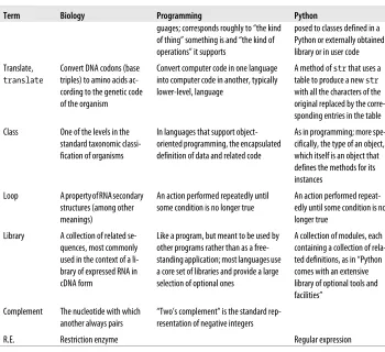
Unfortunate and Unavoidable Vocabulary Overlap

This book’s vocabulary is drawn from three domains that, for the most part, are inde-pendent of each other: computer science (including data structures and programming language concepts), Python (which has its own names for the program and data struc-tures it offers), and biology. Certain words appear in two or even all three of these domains, often playing a major role and having a different meaning in each. The result is unfortunate and unavoidable collisions of vocabulary. Care was taken to establish

(24)

(25)

(26)

Conventions Used in This Book

The following typographical conventions are used in this book:

Italic

Indicates new terms, URLs, filenames, and file extensions, and is used for docu-mentation and comments in code examples

Constant width

Used for names of values, functions, methods, classes, and other code elements, as well as the code in examples, the contents of files, and printed output

Constant width bold

Indicates user input to be typed at an interactive prompt, and highlights Python statement keywords in examples

Constant width italic

Shows text that should be replaced with user-supplied values; also used in exam-ples for “pseudocode” meant to be replaced with actual Python code

This icon signifies a tip, suggestion, or general note.

This icon indicates a warning or caution.

Some chapters include text and code in specially labeled sidebars. These capture ex-planations and examples in an abstract form. They are meant to serve as aids to learning the first time you go through the material, and useful references later. There are three kinds of these special sidebars:

S T A T E M E N T

Every kind of Python statement is explained in text and examples and summarized in a statement box.

S Q L

(27)

T E M P L A T E

In place of theoretical discussions of the many ways a certain kind of code can be written, this book presents generalized abstract patterns that show how such code would typically appear in bioinformatics programs. The idea is that, at least in the early stages of using what you learn in this book, you can use the templates in your programs, replacing the abstract parts with the concrete details of your code.

We’d Like to Hear from You

Every example in this book has been tested, but occasionally you may encounter prob-lems. Mistakes and oversights can occur, and we will gratefully receive details of any that you find, as well as any suggestions you would like to make for future editions. You can contact the author and editor at:

O’Reilly Media, Inc.

1005 Gravenstein Highway North Sebastopol, CA 95472

800-998-9938 (in the United States or Canada) 707-829-0515 (international or local)

707-829-0104 (fax)

We have a web page for this book, where we list errata, examples, and any additional information. You can access this page at:

http://www.oreilly.com/catalog/9780596154509/

To comment or ask technical questions about this book, send email to the following, quoting the book’s ISBN number (9780596154509):

[email protected]

For more information about our books, conferences, Resource Centers, and the O’Reilly Network, see our website at:

http://www.oreilly.com

Using Code Examples

This book is here to help you get your job done. In general, you may use the code in this book in your programs and documentation. You do not need to contact us for permission unless you’re reproducing a significant portion of the code. For example, writing a program that uses several chunks of code from this book does not require permission. Selling or distributing a CD-ROM of examples from O’Reilly books does require permission. Answering a question by citing this book and quoting example

(28)

code does not require permission. Incorporating a significant amount of example code from this book into your product’s documentation does require permission.

We appreciate, but do not require, attribution. An attribution usually includes the title, author, publisher, and ISBN. For example: “Bioinformatics Programming using

If you feel your use of code examples falls outside fair use or the permission given here, feel free to contact us at [email protected].

Safari® Books Online

Safari Books Online is an on-demand digital library that lets you easily search over 7,500 technology and creative reference books and videos to find the answers you need quickly.

With a subscription, you can read any page and watch any video from our library online. Read books on your cell phone and mobile devices. Access new titles before they are available for print, and get exclusive access to manuscripts in development and post feedback for the authors. Copy and paste code samples, organize your favorites, down-load chapters, bookmark key sections, create notes, print out pages, and benefit from tons of other time-saving features.

O’Reilly Media has uploaded this book to the Safari Books Online service. To have full digital access to this book and others on similar topics from O’Reilly and other pub-lishers, sign up for free at http://my.safaribooksonline.com.

Acknowledgments

(29)

I thank my students at Northeastern University’s Professional Masters in Bioinformat-ics program for their patience, suggestions, and error detection while using earlier ver-sions of the book’s text and code. Special thanks go to Jyotsna Guleria, a graduate of that program, who wrote test programs for the example code that uncovered significant latent errors. (Extended versions of the test programs can be found on the book’s website.) Finally, I hope what I have produced justifies what my friends, family, and colleagues endured during its creation—especially Janet, my wife, whose unwavering support during the book’s writing made the project possible.

(30)

(31)

CHAPTER 1

Primitives

Computer programs manipulate data. This chapter describes the simplest kinds of Python data and the simplest ways of manipulating them. An individual item of data is called a value. Every value in Python has a type that identifies the kind of value it is. For example, the type of 2 is int. You’ll get more comfortable with the concepts of types and values as you see more examples.

The Preface pointed out that Python is a multiparadigm programming language. The terms “type” and “value” come from traditional procedural programming. The equiv-alent object-oriented terms are class and object. We’ll mostly use the terms “type” and “value” early on, then gradually shift to using “class” and “object” more frequently. Although Python’s history is tied more to object-oriented programming than to tradi-tional programming, we’ll use the term instance with both terminologies: each value is an instance of a particular type, and each object is an instance of a particular class.

Simple Values

Types for some simple kinds of values are an integral part of Python’s implementation. Four of these are used far more frequently than others: logical (Boolean), integer,

float, and string. There is also a special no-value value called None.

When you enter a value in the Python interpreter, it prints it on the following line:

>>> 90

90 >>>

When the value is None, nothing is printed, since None means “nothing”:

>>> None

>>>

If you type something Python finds unacceptable in some way, you will see a multiline message describing the problem. Most of what this message says won’t make sense

(32)

until we’ve covered some other topics, but the last line should be easy to understand and you should learn to pay attention to it. For example:

>>> Non

Traceback (most recent call last): File "<pyshell#7>", line 1, in <module> Non

NameError: name 'Non' is not defined >>>

When a # symbol appears on a line of code, Python ignores it and the rest of the line. Text following the # is called a comment. Typically comments offer information about the code to aid the reader, but they can include many other kinds of text: a program-mer’s notes to fix or investigate something, a reference (documentation entry, book title, URL, etc.), and so on. They can even be used to “comment out” code lines that are not working or are obsolete but still of interest. The code examples that follow include occasional comments that point out important details.

Booleans

There are only two Boolean values: True and False. Their type is bool. Python names are “case-sensitive,” so true is not the same as True:

>>> True

True >>> False

False

Integers

There’s not much to say about Python integers. Their type is int, and they can have as many digits as you want. They may be preceded by a plus or minus sign. Separators such as commas or periods are not used:

>>> 14

14 >>> −1

−1

>>> 1112223334445556667778889990000000000000 # a very large integer!

1112223334445556667778889990000000000000

Python 2: A distinction is made between integers that fit within a certain (large) range and those that are larger; the latter are a separate type called

long.

(33)

>>> 0x12 # (1 x 16 )+ 2

18

>>> 0xA40 # (10 x 16 x 16) + (4 x 16) + 0

2624

>>> 0xFF # (15 x 16) + 15

255

The result of entering a hexadecimal number is still an integer—the only difference is in how you write it. Hexadecimal notation is used in a lot of computer-related contexts because each hexadecimal digit occupies one half-byte. For instance, colors on a web page can be specified as a set of three one-byte values indicating the red, green, and blue levels, such as FFA040.

Floats

“Float” is an abbreviated version of the term “floating point,” which refers to a number that is represented in computer hardware in the equivalent of scientific notation. Such numbers consist of two parts: digits and an exponent. The exponent is adjusted so the decimal point “floats” to just after the first digit (or just before, depending on the implementation), as in scientific notation.

The written form of a float always contains a decimal point and at least one digit after it:

>>> 2.5

2.5

You might occasionally see floats represented in a form of scientific notation, with the letter “e” separating the base from the exponent. When Python prints a number in scientific notation it will always have a single digit before the decimal point, some number of digits following the decimal point, a + or - following the e, and finally an integer. On input, there can be more than one digit before the decimal point. Regardless of the form used when entering a float, Python will output very small and very large numbers using scientific notation. (The exact cutoffs are dependent on the Python implementation.) Here are some examples:

>>> 2e4 # Scientific notation, but...

20000.0 # within the range of ordinary floats.

>>> 2e-2

0.02

>>>.0001 # Within the range of ordinary floats

0.0001 # so printed as an ordinary float.

>>>.00001 # An innocent-looking float that is

1e-05 # smaller than the lower limit, so e.

>>> 1002003004005000. # A float with many digits that is

1002003004005000.0 # smaller than the upper limit, so no e.

>>> 100200300400500060. # Finally, a float that is larger than the

1.0020030040050006e+17 # upper limit, so printed with an e.

(34)

Strings

Strings are series of Unicode*_{characters. Their type is}_str_{. Many languages have a}

separate “character” type, but Python does not: a lone character is simply a string of length one. A string is enclosed in a pair of single or double quotes. Other than style preference, the main reason to choose one or the other kind of quote is to make it convenient to include the other kind inside a string.

If you want a string to span multiple lines, you must enclose it in a matched pair of three single or double quotes. Adding a backslash in front of certain characters causes those characters to be treated specially; in particular, '\n' represents a line break and '\t' represents a tab.

Python 2: Strings are composed of one-byte characters, not Unicode characters; there is a separate string type for Unicode, designated by preceding the string’s opening quote with the character u.

We will be working with strings a lot throughout this book, especially in representing DNA/RNA base and amino acid sequences. Here are the amino acid sequences for some unusually small bacterial restriction enzymes:†

>>> 'MNKMDLVADVAEKTDLSKAKATEVIDAVFA'

MNKMDLVADVAEKTDLSKAKATEVIDAVFA

>>> "AARHQGRGAPCGESFWHWALGADGGHGHAQPPFRSSRLIGAERQPTSDCRQSLQQSPPC"

AARHQGRGAPCGESFWHWALGADGGHGHAQPPFRSSRLIGAERQPTSDCRQSLQQSPPC

>>> """MKQLNFYKKN SLNNVQEVFS YFMETMISTN RTWEYFINWD KVFNGADKYR NELMKLNSLC GS LFPGEELK SLLKKTPDVV KAFPLLLAVR DESISLLD"""

'MKQLNFYKKN SLNNVQEVFS YFMETMISTN RTWEYFINWD KVFNGADKYR NELMKLNSLC GS LFPGEELK\nSLLKKT PDVV KAFPLLLAVR DESISLLD'

>>> '''MWNSNLPKPN AIYVYGVANA NITFFKGSDI LSYETREVLL KYFDILDKDE RSLKNALKD LEN PFGFAPYI RKAYEHKRNF LTTTRLKASF RPTTF'''

'MWNSNLPKPN AIYVYGVANA NITFFKGSDI LSYETREVLL KYFDILDKDE RSLKNALKDL EN\nPFGF APYI RKAYEHKRNF LTTTRLKASF RPTTF'

There are three situations that cause input or output to begin on a new line: • You hit Return as you are typing inside a triple-quoted string.

• You keep typing characters until they “wrap around” to the next line before you press Return.

• The interpreter responds with a string that is too long to fit on one line.

* Unicode characters occupy between one and four bytes each in memory, depending on several factors. See http://docs.python.org/3.1/howto/unicode.html for details (in particular, http://docs.python.org/3.1/howto/ unicode.html#encodings). For general information about Unicode outside of Python, consult http://www .unicode.org/standard/WhatIsUnicode.html, http://www.unicode.org/standard/principles.html, and http:// www.unicode.org/resources.

(35)

Only the first one is “real.” The other two are simply the effect of output “line wrapping” like what you would see in text editors or email programs. In the second and third situations, if you change the width of the window the input and output strings will be “rewrapped” to fit the new width. The first case does not cause a corresponding line break when the interpreter prints the string—the Return you typed becomes a '\n' in the string.

Normally, Python uses a pair of single quotes to enclose strings it prints. However, if the string contains single quotes (and no double quotes), it will use double quotes. It never prints strings using triple quotes; instead, the line breaks typed inside the string become '\n's.

Expressions

An operator is a symbol that indicates a calculation using one or more operands. The combination of the operator and its operand(s) is an expression.

Numeric Operators

A unary operator is one that is followed by a single operand. A binary operator is one that appears between two operands. It isn’t necessary to surround operators with spaces, but it is good style to do so. Incidentally, when used in a numeric expression, False is treated as 0 and True as 1.

Plus and minus can be used as either unary or binary operators:

>>> −1 # unary minus

-1 >>> 4 + 2

6 >>> 4 − 1

3 >>> 4 * 3

12

The power operator is ** (i.e., nk_{is written}_{n ** k}_):

>>> 2 ** 10

1024

There are three operators for the division of one integer by another: / produces a float, // (floor division) an integer with the remainder ignored, and % (modulo) the remainder of the floor division. The formal definition of floor division is “the largest integer not greater than the result of the division”:

>>> 11 / 4

2.75

>>> 11 // 4 # "floor" division

2

(36)

>>> 11 % 4 # remainder of 11 // 3

3

Python 2: The / operator performs floor division when both operands are ints, but ordinary division if one or both operands are floats.

Whenever one or both of the operators in an arithmetic expression is a float, the result will be a float:

>>> 2.0 + 1

3.0

>>> 12 * 2.5

30.0 >>> 7.5 // 2

3.0

While the value of floor division is equal to an integer value, its type may

not be integer! If both operands are ints, the result will be an int, but if either or both are floats, the result will be a float that represents an integer.

The result of an operation does not always print the way you might expect. Consider the following numbers:

>>> .009

.009 >>> .01

.01 >>> .029

.029 >>> .03

.03 >>> .001

.001

So far, everything is as expected. If we subtract the first from the second and the third from the fourth, we should in both cases get the result .001. Typing in .001 also gives the expected result. However, typing in the subtraction operations does not:

>>> .03 - .029

0.0009999999999999974 >>> .01 - .009

0.0010000000000000009

Strange results like this arise from two sources:

(37)

• A computer stores rational numbers in a finite number of binary digits; the binary representation of a rational number may in fact have an exact binary representa-tion, but one that would require more digits than are used.

A rational number is one that can be expressed as a/b, where b is not zero; the decimal-point expression of a rational number in a given num-ber system either has a finite numnum-ber of digits or ends with an infinitely repeating sequence of digits. There’s nothing wrong with the binary system: whatever base is used, some real numbers have exact represen-tations and others don’t. Just as only some rational numbers have exact decimal representations, only some rational numbers have exact binary representations.

As you can see from the results of the two division operations, the difference between the ideal rational number and its actual representation is quite small, but in certain kinds of computations the differences do accumulate.‡

Here’s an early lesson in an extremely important programming principle: don’t trust

what you see! Everything printed in a computing environment or by a programming

language is an interpretation of an internal representation. That internal representation may be manipulated in ways that are intended to be helpful but can be misleading. In the preceding example, 0.009 in fact does not have an exact binary representation. In Python 2, it would have printed as 0.0089999999999999993, and 0.003 would have prin-ted as 0.0089999999999999993. The difference is that Python 3 implements a more so-phisticated printing mechanism for rational numbers that makes some of them look as they would have had you typed them.

Logical Operations

Python, like other programming languages, provides operations on “truth values.” These follow the mathematical laws of Boolean logic. The classic Boolean operators are not, and, and or. In Python, those are written just that way rather than using special symbols:

>>> not True

False >>> not False

True

>>> True and True

True

>>> True and False

False

>>> True or True

True

‡ A computer science field called “numerical analysis” provides techniques for managing the accumulation of such errors in complex or repetitive computations.

(38)

>>> True or False

True

>>> False and False

False

>>> False or True

The results of and and or operations are not converted to Booleans. For

and expressions, the first operand is returned if it is false; otherwise, the second operand is returned. For or expressions, the first operand is re-turned if it is true; otherwise, the second operand is rere-turned. For example:

>>> '' and 'A'

'' # Not False: '' is a false value

>>> 0 and 1 or 2 # Read as (0 and 1) or 2

2 # Not True: 2 is a false value

While confusing, this can be useful; we’ll see some examples later.

The operands of and and or can actually be anything. None, 0, 0.0, and the empty string, as well as the other kinds of “empty” values explained in Chapter 3, are considered False. Everything else is treated as True.

To avoid repetition and awkward phrases, this book will use “true” and “false” in regular typeface to indicate values considered to be True and

False, respectively. It will only use the capitalized words True and

False in the code typeface when referring to those specific Boolean values.

There is one more logical operation in Python that forms a conditional expression. Written using the keywords if and else, it returns the value following the if when the condition is true and the value following the else when it is false. We’ll look at some more meaningful examples a bit later, but here are a few trivial examples that show what conditional expressions look like:

>>> 'yes' if 2 - 1 else 'no'

'yes'

>>> 'no' if 1 % 2 else 'no'

'no'

In addition to the Boolean operators, there are six comparison operators that return Boolean values: ==, !=, <, <=, >, and >=. These work with many different kinds of operands:

>>> 2 == 5 // 2

True

>>> 3 > 13 % 5

False

>>> 'one' < 'two'

(39)

>>> 'one' != 'one'

False

You may already be familiar with logical and comparison operations from other com-puter work you’ve done, if only entering spreadsheet formulas. If these are new to you, spend some time experimenting with them in the Python interpreter until you become comfortable with them. You will use them frequently in code you write.

String Operations

There are four binary operators that act on strings: in, not in, +, and *. The first three expect both operands to be strings. The last requires the other operator to be an integer. A one-character substring can be extracted with subscription and a longer substring by slicing. Both use square brackets, as we’ll see shortly.

String operators

The in and not in operators test whether the first string is a substring of the second one (starting at any position). The result is True or False:

>>> 'TATA' in 'TATATATATATATATATATATATA'

True

>>> 'AA' in 'TATATATATATATATATATATATA'

False

>>> 'AA' not in 'TATATATATATATATATATATATA'

True

A new string can be produced by concatenating two existing strings. The result is a string consisting of all the characters of the first operand followed by all the characters of the second. Concatenation is expressed with the plus operator:

>>> 'AC' + 'TG'

'ACTG'

>>> 'aaa' + 'ccc' + 'ttt' + 'ggg'

'aaaccctttggg'

A string can be repeated a certain number of times by multiplying it by an integer:

>>> 'TA' * 12

'TATATATATATATATATATATATA' >>> 6 * 'TA'

'TATATATATATA'

Subscription

Subscription extracts a one-character substring of a string. Subscription is expressed

with a pair of square brackets enclosing an integer-valued expression called an index. The first character is at position 0, not 1:

>>> 'MNKMDLVADVAEKTDLSKAKATEVIDAVFA'[0]

'M'

'N'

(40)

The index can also be negative, in which case the index is counted from the end of the string. The last character is at index −1:

>>> 'MNKMDLVADVAEKTDLSKAKATEVIDAVFA'[−1]

'A'

>>> 'MNKMDLVADVAEKTDLSKAKATEVIDAVFA'[−5]

'D'

>>> 'MNKMDLVADVAEKTDLSKAKATEVIDAVFA'[7 // 2]

'K'

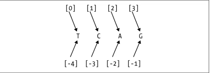
As Figure 1-1 shows, starting at 0 from the beginning or end of a string, an index can be thought of as a label for the character to its right. The end of a string is the position one after the last element. If you are unfamiliar with indexing in programming lan-guages, this is probably an easier way to visualize it than if you picture the indexes as aligned with the characters.

Figure 1-1. Index positions in strings

Attempting to extract a character before the first or after the last causes an error, as shown here:

Traceback (most recent call last): File "<pyshell#14>", line 1, in <module> 'MNKMDLVADVAEKTDLSKAKATEVIDAVFA'[50] IndexError: string index out of range

The last line reports the nature of the error, while the next-to-last line shows the input that caused the error.

Slicing

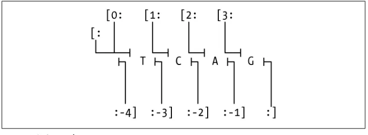
Slicing extracts a series of characters from a string. You’ll use it often to clearly and

concisely designate parts of strings. Figure 1-2 illustrates how it works.

(41)

character m up to but not including character n.” (We’ll explore the use of the third index momentarily). Here are a few slicing examples:

>>> 'MNKMDLVADVAEKTDLSKAKATEVIDAVFA'[1:4]

'NKM'

>>> 'MNKMDLVADVAEKTDLSKAKATEVIDAVFA'[4:-1]

'DLVADVAEKTDLSKAKATEVIDAVF'

>>> 'MNKMDLVADVAEKTDLSKAKATEVIDAVFA'[-5:-4]

'D'

Either of the indexes can be positive, indicating “from the beginning,” or negative, indicating “from the end.” If neither of the two numbers is negative, the length of the resulting string is the difference between the second and the first. If either (or both) is negative, just add it to the length of the string to convert it to a nonnegative number. What if the two numbers are the same? For example:

>>> 'MNKMDLVADVAEKTDLSKAKATEVIDAVFA'[5:5]

''

Since this reads as “from character 5 up to but not including character 5,” the result is an empty string. Now, what about character positions that are out of order—i.e., where the first character occurs after the second? This results in an empty string too:

>>> 'MNKMDLVADVAEKTDLSKAKATEVIDAVFA'[-4:-6]

''

For subscription, the index must designate a character in the string, but the rules for slicing are less constraining.

When the slice includes the beginning or end of the string, that part of the slice notation may be omitted. Note that omitting the second index is not the same as providing −1 as the second index—omitting the second index says to go up to the end of the string, one past the last character, whereas −1 means go up to the penultimate character (i.e., up to but not including the last character):

>>> 'MNKMDLVADVAEKTDLSKAKATEVIDAVFA'[:8]

'MNKMDLVADVAEKTDLSKAKAT'

>>> 'MNKMDLVADVAEKTDLSKAKATEVIDAVFA'[9:] Figure 1-2. String slicing

(42)

'VAEKTDLSKAKATEVIDAVFA'

>>> 'MNKMDLVADVAEKTDLSKAKATEVIDAVFA'[9:-1]

'VAEKTDLSKAKATEVIDAVF'

In fact, both indexes can be omitted, in which case the entire string is selected:

>>> 'MNKMDLVADVAEKTDLSKAKATEVIDAVFA'[:]

'MNKMDLVADVAEKTDLSKAKATEVIDAVFA'

Finally, as mentioned earlier, a slice operation can specify a third number, also follow-ing a colon. This indicates a number of characters to skip after each one that is included, known as a step. When the third number is omitted, as it often is, the default is 1, meaning don’t skip any. Here’s a simple example:

>>> 'MNKMDLVADVAEKTDLSKAKATEVIDAVFA'[0:9:3]

'MMV'

This example’s result was obtained by taking the first, fourth, and seventh characters from the string. The step can be also be a negative integer. When the step is negative, the slice takes characters in reverse order. To get anything other than an empty string when you specify a negative step, the start index must be greater than the stop index:

>>> 'MNKMDLVADVAEKTDLSKAKATEVIDAVFA'[16:0:-4]

'SKDD'

Notice that the first character of the string is not included in this example’s results. The character at the stop index is never included. Omitting the second index so that it defaults to the beginning of the string—beginning, not end, because the step is negative—results in a string that does include the first character, assuming the step would select it. Changing the previous example to omit the 0 results in a longer string:

>>> 'MNKMDLVADVAEKTDLSKAKATEVIDAVFA'[16::-4]

'SKDDM'

Omitting the first index when the step is negative means start from the end of the string:

>>> 'MNKMDLVADVAEKTDLSKAKATEVIDAVFA'[:25:-1]

'AFVA'

A simple but nonobvious slice expression produces a reversed copy of a string:

s[::-1]. This reads as “starting at the end of the string, take every character up to and

including the first, in reverse order”:

>>> 'MNKMDLVADVAEKTDLSKAKATEVIDAVFA'[::-1]

'AFVADIVETAKAKSLDTKEAVDAVLDMKNM'

Calls

We’ll look briefly at calls here, deferring details until later. A call is a kind of expression.

Function calls

The simplest kind of call invokes a function. A call to a function consists of a function

(43)

commas. The function is called, does something, then returns a value. Before the func-tion is called the argument expressions are evaluated, and the resulting values are

passed to the function to be used as input to the computation it defines. An argument

can be any kind of expression whose result has a type acceptable to the function. Those expressions can also include function calls.

Each function specifies the number of arguments it is prepared to receive. Most func-tions accept a fixed number—possibly zero—of arguments. Some accept a fixed num-ber of required arguments plus some numnum-ber of optional arguments. We will follow the convention used in the official Python documentation, which encloses optional arguments in square brackets. Some functions can even take an arbitrary number of arguments, which is shown by the use of an ellipsis.

Python has a fairly small number of “built-in” functions. Some of the more frequently used are:

len(arg)

Returns the number of characters in arg (although it’s actually more general than that, as will be discussed later)

print(args...[, sep=seprstr][, end=endstr])

Prints the arguments, of which there may be any number, separating each by a seprstr (default ' ') and omitting certain technical details such as the quotes sur-rounding a string, and ending with an endstr (default '\n')

Python 2: print is a statement, not a function. There is no way to specify a separator. The only control over the end is that a final comma sup-presses the newline.

input(string)

Prompts the user by printing string, reads a line of input typed by the user (which ends when the Return or Enter key is pressed), and returns the line as a string

Python 2: The function’s name is raw_input.

Here are a few examples:

>>> len('TATA')

4

>>> print('AAT', 'AAC', 'AAG', 'AAA')

AAT AAC AAG AAA

>>> input('Enter a codon: ')

Enter a codon: CGC

'CGC' >>>

(44)

Here are some common numeric functions in Python: abs(value)

Returns the absolute value of its argument max(args...)

Returns the maximum value of its arguments min(args...)

Returns the minimum value of its arguments

Types can be called as functions too. They take an argument and return a value of the type called. For example:

str(arg)

Returns a string representation of its argument int(arg)

Returns an integer derived from its argument float(arg)

Returns a float derived from its argument bool(arg)

Returns False for None, zeros, empty strings, etc., and True otherwise; rarely used, because other types of values are automatically converted to Boolean values wherever Boolean values are expected

Here are some examples of these functions in action:

>>> str(len('TATA'))

'4'

>>> int(2.1)

2

>>> int('44')

44

>>> bool('')

False >>> bool(' ')

True >>> float(3)

3.0

Using int is the only way to guarantee that the result of a division is an integer. As noted earlier, // is the floor operator and results in a float if either operand is a float.

(45)

help()

Enters the interactive help facility help(x)

Prints information about x, which can be anything (a value, a type, a function, etc.); help for a type generally includes a long list of things that are part of the type’s implementation but not its general use, indicated by names beginning with underscores

Occasionally your code needs to test whether a value is an instance of a certain type; for example, it may do one thing with strings and another with numbers. You can do this with the following built-in function:

isinstance(x,sometype)

Returns True if x is an instance of the type (class) sometype, and False otherwise

Method calls

Many different types of values can be supplied as arguments to Python’s built-in func-tions. Most functions, however, are part of the implementation of a specific type. These are called methods. Calling a method is just like calling a function, except that the first argument goes before the function name, followed by a period. For example, the method count returns the number of times its argument appears in the string that pre-cedes it in the call. The following example returns 2 because the string 'DL' appears twice in the longer string:

>>> 'MNKMDLVADVAEKTDLSKAKATEVIDAVFA'.count('DL')

2

Except for having their first argument before the function name, calls to methods have the same features as calls to ordinary functions: optional arguments, indefinite number of arguments, etc. Here are some commonly used methods of the str type:

string1.count(string2[,start[,end]])

Returns the number of times string2 appears in string1. If start is specified, starts counting at that position in string1; if end is also specified, stops counting before that position in string1.

string1.find(string2[,start[,end]])

Returns the position of the last occurrence of string2 in string1; −1 means string2 was not found in string1. If start is specified, starts searching at that position in string1; if end is also specified, stops searching before that position in string1.

string1.startswith(string2[,start[,end]])

Returns True or False according to whether string2 starts with string1. If start is specified, uses that as the position at which to start the comparison; if end is also specified, stops searching before that position in string1.

(46)

string1.strip([string2])

Returns a string with all characters in string2 removed from its beginning and end; if string2 is not specified, all whitespace is removed.

string1.lstrip([string2])

Returns a string with all characters in string2 removed from its beginning; if string2 is not specified, all whitespace is removed.

string1.rstrip([string2])

Returns a string with all characters in string2 removed from its end; if string2 is not specified, all