ABSTRACT
KHADE, AJINKYA SANJAY. Gait Phase Parameter Estimation and Model Predictive Control of Active Transfemoral Prosthesis. (Under the direction of Dr. Fen Wu.)
© Copyright 2016 by Ajinkya Sanjay Khade
Gait Phase Parameter Estimation and Model Predictive Control of Active Transfemoral Prosthesis
by
Ajinkya Sanjay Khade
A thesis submitted to the Graduate Faculty of North Carolina State University
in partial fulfillment of the requirements for the Degree of
Master of Science
Mechanical Engineering
Raleigh, North Carolina
2016
APPROVED BY:
Dr. Aranya Chakrabortty Minor Advisor
Dr. Gregory Buckner
Dr. Fen Wu
DEDICATION
BIOGRAPHY
ACKNOWLEDGEMENTS
The two years of graduate school at North Carolina State University have been a huge learning experience for me. I feel confident that everything I have learned here is going to help me in the grand scheme of things, even if it might not be obvious right now how all the dots connect. And for that I have a lot of people to thank. First and foremost, I would like to thank my advisor Dr. Fen Wu for giving me the chance to work under his guidance. His insightful approach and wise judgment have helped me navigate the tricky waters of conducting research. His help with my technical problems and his patience while I dealt with personal matters have gone a long way in making my experience during this journey enjoyable. But most importantly, I would like to thank him for introducing me to this domain. The work I have done has strengthened my interest in this field of work while also helping me to expand my horizons. This interest in allied fields lead me to apply for a minor in Electrical Engineering.
I would like to thank Dr. Aranya Chakrabortty for serving as myMinor Advisor. The courses he helped me choose for my minor have complimented my domain knowledge very well, and have provided me with a very broad background. This has allowed me to take a very holistic view of all technical problems and tackle them with a unique perspective. The course taught by him has helped me a lot in my research while also giving me a taste of real-world problems. I am grateful to Dr. Gregory Buckner for serving on my committee. His course has been one of the most enjoyable ones during my Masters, and his guidance and support have proven to be valuable in this endeavor.
to approach learning. I am also thankful to my peers and lab mates. Watching them excel in their endeavors has motivated me to set a high bar for myself and to constantly push myself.
As important as academic endeavors are for success, their true value can be achieved only in conjunction with personal development. And while it can be difficult to maintain the balance between work and personal life in graduate school, family and friends make it a little easier. I have been blessed to have great friends over the course of my life and their help and support is a big factor that has kept me going.
Everyone has role models that they look up to, and I am no different in that regard. Growing up in a nation where cricket is not merely a sport but very much a religion, Sachin Tendulkar - its foremost protagonist - has had a deep influence on me. Watching him wield his magic on the field has given me pleasure very few things can, and has helped me get through some tough days. But the more important lessons I have learned by watching him are the value of humility, dedication and hard work. He has taught me that no amount of talent or skill can make up for the value of hard work; and if you set your mind to it, nothing is impossible. And I will be forever grateful for these values.
TABLE OF CONTENTS
LIST OF TABLES . . . viii
LIST OF FIGURES. . . ix
Chapter 1 Introduction. . . 1
1.1 Types of Knee Prosthesis . . . 2
1.2 Control of Prosthesis . . . 4
1.3 Why MPC . . . 5
1.4 Proposed Solution . . . 6
Chapter 2 Fundamentals of ATP . . . 7
2.1 Experimental Setup . . . 8
2.1.1 Prototype Construction . . . 8
2.1.2 Knee Impedance Control . . . 9
2.1.3 Gait Modes . . . 10
2.1.4 Data Collection . . . 12
2.2 Gait Modeling . . . 13
2.2.1 Assumptions . . . 14
2.2.2 Problem Formulation . . . 14
2.2.3 ODE Gait Model . . . 16
Chapter 3 Parameter Estimation. . . 18
3.1 Motivations and Objectives . . . 19
3.2 Overview . . . 20
3.3 Problem Formulation . . . 22
3.3.1 Terminology Used . . . 22
3.3.2 Optimization Parameters . . . 25
3.3.3 Constraints . . . 26
3.3.4 Weighted Parameters . . . 27
3.3.5 Cost Function . . . 28
3.4 Optimization Strategies . . . 29
3.4.1 Differential Equation Solver Method . . . 30
3.4.2 Discrete Optimization Method . . . 33
3.5 Optimization Roadmap . . . 35
3.6 Implementation Details . . . 38
3.6.1 Choice of Solver . . . 39
3.6.2 Initial Estimate . . . 40
3.6.3 Parameter Weights . . . 41
3.7 Discussion of Results . . . 44
3.7.1 Subject Parameter Estimates . . . 44
3.7.2 Analysis of Results . . . 44
Chapter 4 Control Design . . . 51
4.1 Motivations and Objectives . . . 52
4.2 Guiding Principle . . . 53
4.3 Problem Formulation . . . 54
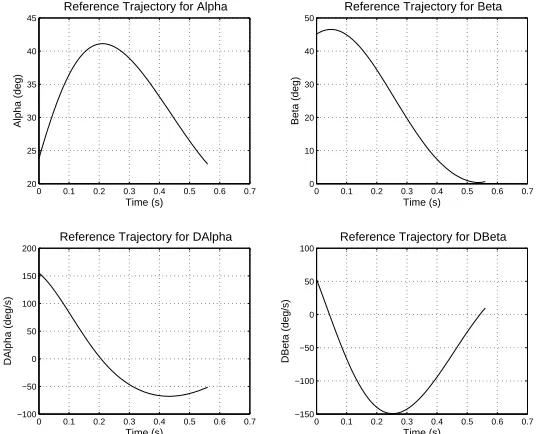
4.3.1 Reference Trajectory . . . 55
4.3.2 Manipulated Variables . . . 55
4.3.3 Output Variables . . . 56
4.3.4 Plant Model . . . 57
4.3.5 Switching Logic . . . 58
4.4 Design Implementation . . . 60
4.4.1 Basics of MPC Theory . . . 60
4.4.2 Sampling Time . . . 62
4.4.3 Prediction Horizon (Np ) . . . 62
4.4.4 Control Horizon (Nc ) . . . 63
4.4.5 Online Optimization Cost . . . 63
4.4.6 Number of Controllers . . . 66
4.4.7 Simulating Prosthesis System Output . . . 67
4.5 Results . . . 68
4.5.1 Baseline Scenario . . . 68
4.5.2 Disturbance Rejection . . . 75
4.5.3 Variation in Number of Controllers . . . 78
4.5.4 Variation in Prediction Horizon . . . 78
4.5.5 Variation in Relative Weights of Output Variables . . . 78
4.5.6 Variation in Relative Weights of Manipulated Variables . . . 82
4.5.7 Effect of Parameter Uncertainty . . . 83
4.5.8 Concluding Remarks . . . 85
Chapter 5 Conclusion . . . 86
5.1 Summary and Novel Contributions . . . 86
5.2 Future Work . . . 91
LIST OF TABLES
Table 3.1 Reference Values for Optimization Parameter Weights . . . 42 Table 3.2 Final estimates of Subject Parameters . . . 45
LIST OF FIGURES
Figure 2.1 Solidworks model of prototype (left); Experimental setup for healthy subject (center); Experimental setup for Transfemoral amputee (right).
Adapted from[Liu14]. . . 9
Figure 2.2 Control Architecture of ATP Prototype . . . 11
Figure 2.3 Gait Modes . . . 12
Figure 2.4 Biped Model . . . 15
Figure 3.1 Simulation offlexion phasewith estimated parameters . . . 47
Figure 3.2 Simulation ofextension phasewith estimated parameters . . . 49
Figure 4.1 Reference Trajectory for Model Predictive Controller . . . 56
Figure 4.2 Basic concept of Model Predictive Control. Adapted from[Seb11] . . 61
Figure 4.3 Simulink Model of the Control Architecture of Prosthesis System . . . 68
Figure 4.4 Simulation of Baseline Scenario with SW1 . . . 71
Figure 4.5 Switching Signal for Baseline Scenario with SW1 . . . 72
Figure 4.6 Simulation of Baseline Scenario with SW2 . . . 73
Figure 4.7 Phase plot for Baseline Scenario with SW2 . . . 74
Figure 4.8 Phase plot for Baseline Scenario with SW1 . . . 74
Figure 4.9 Time response plot when disturbance is applied at t=0.2 s . . . 76
Figure 4.10 Phase plot when disturbance is applied at t=0.2 s . . . 77
Figure 4.11 Comparison of Switching signal when disturbance is applied at t=0.2 s 77 Figure 4.12 Time response plot for varying of number of controllers . . . 79
Figure 4.13 Phase plot for varying of number of controllers . . . 80
Figure 4.14 Phase plot for varying prediction horizon . . . 80
Figure 4.15 Time response plot for varying relative weight ofβ . . . 81
Figure 4.16 Phase plot for varying relative weight ofβ . . . 82
Figure 4.17 Phase plot for varying relative weight ofτhip . . . 83
CHAPTER
1
INTRODUCTION
Limb loss has devastating effects on any individual who has the misfortune of experiencing it. The problem is much greater if the limb lost is a lower limb. Locomotion is key to any human endeavor and this ability is something most individuals take for granted. When that is impaired, it reduces a person’s independence and affects their quality of life.
1.1. TYPES OF KNEE PROSTHESIS CHAPTER 1. INTRODUCTION
expected to double by 2050. It is difficult to find the equivalent worldwide statistics, since many countries do not keep a record of amputees or cause and level of amputation. Clearly, this is a problem that deserves a lot of attention and resources.
1.1
Types of Knee Prosthesis
The loss of knee joint dramatically reduces the way an individual can manipulate any prosthesis. Quite a few prosthetic devices have been developed over the years which try to improve the quality of life for amputees. Most of these devices make it possible for the amputee to walk again on level-ground, although they require varying levels of training and energy. These knee prostheses can be divided into three categories[Har13],[SP09]
1. Mechanically Passive Prostheses
-As the name suggests, these devices are energetically passive and provide no net power input. The movement of the joints relies on the properties of its mechanical components. And although no sensors are required, the users must perform com-pensatory movements with their other body parts such as trunk and residual limb. Such devices require a large amount of energy from the user and greatly restrict the types of maneuvers they can perform.
2. MicroprocessorControlled Mechanically Passive Prosthesis
1.1. TYPES OF KNEE PROSTHESIS CHAPTER 1. INTRODUCTION
The advantages include greater flexibility, ability to adapt to different walking speeds and greater knee stability. They also reduce the amputee energy consumption and improve smoothness of gait. Although these devices carry on-board power for sensors and modulating impedance, they still can not produce net positive mechanical power. This remains a big limiting factor that impairs their ability to perform maneuvers like sit-to-stand, and climbing up slopes or stairs, which require net positive power input at some or all of the joints.
3. MicroprocessorControlled Mechanically Active Devices
-The limitations of the mechanically passive types have lead to a lot of interest in developing a self-contained powered prosthesis that is humanlike in its physical characteristics while being energetically efficient. These devices use a higher level control strategy similar to that of the previous types. Gait cycle is divided in different phases and sensory information is used to determine current phase. A lower-level controller then calculates the joint torques that are required in order to mimic natural gait. Different types of designs have been proposed for this class of prosthesis. One of them[Rou13]tries to leverage the passive dynamics of the leg more like a human muscle does. However some variation of the design proposed by[Sup08]has proven to be popular among researchers, by virtue of having a similar mechanical structure to a human leg.
1.2. CONTROL OF PROSTHESIS CHAPTER 1. INTRODUCTION
1.2
Control of Prosthesis
Once the mechanical design of prosthesis is finalized, an appropriate control algorithm needs to be designed. Without a suitable control scheme, it can be very tough to perform regular walking maneuvers. This research area has received a lot of attention lately.
Most of the current control schemes tend to use Finite-State Impedance Control. This scheme uses the same higher-level architecture described previously, where the current state (gait phase) of the system is detected first. This division of gait cycle into different phases or modes will be elaborated upon in subsection 2.1.3. Within each phase, the control law is modeled like a passive spring damper system. The mechanical impedance of this spring damper system is tuned such that the prosthetic leg closely mimics the motion of a human knee. This form of control will be explored in further detail in subsection 2.1.2.
1.3. WHY MPC CHAPTER 1. INTRODUCTION
and uncertain scenarios.
All these reasons mean that a lot is left to be addressed in terms of improving the quality of life for amputees. This prompts the need for a model based control scheme that is designed using an accurate model of gait dynamics.
1.3
Why MPC
Model Predictive Control (MPC)is an advanced algorithm that calculates the control input by predicting how the system states will evolve with time. MPC achieves this by solving an online optimization problem and calculating the optimal control input required to track any given reference trajectory.
However, this requires an accurate mathematical model of the system. Since the gait dynamics model is highly nonlinear, solving nonlinear constraints in real time for fast evolv-ing processes can prove to be challengevolv-ing, and requires a large amount of computational resources. For this reason, the MPC has traditionally been used for slow and stationary processes such as controlling a chemical plant. However, with the explosion in availability of cheap and powerful microprocessors, this constraint is fading away very quickly.
1.4. PROPOSED SOLUTION CHAPTER 1. INTRODUCTION
1.4
Proposed Solution
The thesis seeks to provide a framework for designing a Model Predictive Controller for Active Transfemoral Prosthesis. In order to do this, however, some reference data is needed for conventional prostheses. This data will be used for validating the gait model and control design. The experimental setup and data collection methodology will be first explained in chapter 2. A brief summary of the model derivation process will then be presented, along with the final gait model used.
However, this model of the gait dynamics has some parameters that are not directly measurable, but are inherent to the system. Phase 1 of the research focuses on estimating these parameters and validating the obtained results. An optimization framework has been presented for carrying out this parameter estimation.
Once reasonable degree of confidence can be expressed in the estimated parameters, the research moves on to Phase 2. This phase focuses on the design of the Model Predictive Controller for mimicking a human knee. The results will then be analyzed to determine the most important factors affecting the performance of the controller.
CHAPTER
2
FUNDAMENTALS OF ATP
2.1. EXPERIMENTAL SETUP CHAPTER 2. FUNDAMENTALS OF ATP
work was originally performed by other researchers and subsequently presented in papers which have been cited at relevant places in this chapter. Nevertheless, explaining how the elements of their research were adapted in the present context is essential to understanding the novel work presented in this thesis.
2.1
Experimental Setup
The data used for this research was collected in experiments performed by Liuet aland presented in[Liu14]. A brief summary of the relevant aspects of the experimental setup and data collection methods is now provided. Further details can be found in the paper cited above.
2.1.1
Prototype Construction
The objective of the ATP prototype was to mimic the biomechanics of human knees as best as possible. Off-the-shelf components were used in order to be able to prototype quickly. Thus, all the actuators and sensors are not necessarily as high-accuracy as may be available in a commercial prosthetic device. This prototype can either be worn directly by an amputee, or by a healthy individual with the help of a bypass adapter. The prototype design and experimental setup has been depicted in Fig. 2.1.
2.1. EXPERIMENTAL SETUP CHAPTER 2. FUNDAMENTALS OF ATP
Figure 2.1Solidworks model of prototype (left); Experimental setup for healthy subject (center); Experimental setup for Transfemoral amputee (right). Adapted from[Liu14]
Ground Reaction Force (GRF) was measured by a load cell attached below the knee unit. This prototype did not have an actuated ankle joint. Although it is desirable to be able to manipulate the ankle joint since it provides an extra degree of freedom, this experimental setup can still provide adequate evidence as to whether the proposed algorithm is a feasible and practical solution. The effect of the presence of an actuated ankle joint on the results obtained will also be explained later.
2.1.2
Knee Impedance Control
The ATP prototype usesFinite-State Impedance Controlin order to produce the desired effect at the knee joint. As explained previously,Impedance Controlhas proven to be a popular choice among researchers in recent years. This is because it provides the user with a way to interact with the prosthesis that is predictable and similar to human gait[MM80].
2.1. EXPERIMENTAL SETUP CHAPTER 2. FUNDAMENTALS OF ATP
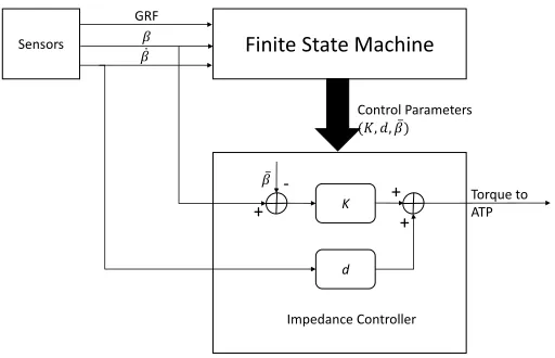
greater detail in subsection 2.1.3. It has been proven using regression analysis of gait data that knee torques can be adequately characterized in the form of passive spring and damper behavior within each of these states. The torque within these states can be expressed in the form
-τknee =K ·(β(t)−β¯) +d·β˙(t) (2.1)
where,K =linear knee stiffness
d =linear knee damping ¯
β=equilibrium angle for current state
The parameters (K,d, ¯β)are collectively referred to as Control Parameters. If they are constrained to be positive, the spring-damper system is guaranteed to be passive, and the joint angleβshould converge to the stable equilibrium ¯β.
Before the ATP can be put into regular use, these control parameters need to be tuned carefully for each state such that the controller mimics a human knee well enough. A procedure similar to [Liu14], [Sup09]can be adopted for this purpose. During regular operation, the finite state machine first detects the current state depending on the sensory measurements and selects the control parameters to be used. The controller then uses these control parameters and the measured values ofβ and ¯βto compute the torque that needs to be applied. This control architecture has been depicted in Fig. 2.2.
2.1.3
Gait Modes
2.1. EXPERIMENTAL SETUP CHAPTER 2. FUNDAMENTALS OF ATP
K
d
Impedance Controller
ҧ
𝛽
-+ + +
Torque to ATP
Finite State Machine
Control Parameters
(𝐾, 𝑑, ҧ𝛽)
Sensors
GRF 𝛽
ሶ
𝛽
Figure 2.2Control Architecture of ATP Prototype
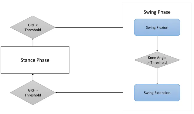
number of gait modes required is not unique, and some different approaches have been previously[Liu14],[Zla02]proposed. The cycle can be broadly divided into two phases - (a) Stance Phaseand (b)Swing Phase.
Gait Cycle starts with the stance phase when the leading foot touches the ground, and continues till it is in contact with the ground. The swing phase starts when this foot, which is now trailing, leaves the ground. This event is known as’toe-off’and is used as the dividing point between stance and swing phase. The swing phase again comes to an end when this foot touches the ground again, known as’heel-strike’.
Various methods have been used by different researchers for further dividing the stance phase into sub-modes. From a clinical gait analysis standpoint, it can be divided into three sub-modes. However, this research only focuses on designing a controller for the swing phase of the gait cycle and thus this subdivision of stance does not need to be explored.
2.1. EXPERIMENTAL SETUP CHAPTER 2. FUNDAMENTALS OF ATP
mode andswing extensionmode. GRF sensor measurements are used to detecttoe-off. GRF magnitude falling below a threshold marks the start of swing flexion. Swing extension starts and swing flexion ends when the shank starts its forward swing, and is characterized by knee angle reaching a specified threshold value. Swing phase ends when GRF magnitude goes above its threshold, marking aheel-strike. The subdivision of gait can be visualized as depicted in Fig. 2.3.
Stance Phase
GRF < Threshold
GRF > Threshold
Knee Angle > Threshold Swing Flexion
Swing Extension
Swing Phase
Figure 2.3Gait Modes
2.1.4
Data Collection
2.2. GAIT MODELING CHAPTER 2. FUNDAMENTALS OF ATP
20 s and then held constant. Data collected over multiple cycles was averaged in order to remove the effect of minor intra-subject variations or measurement errors. Further details of the data collection methodologies can be found in[Liu14].
Theshank massandshank inertiain the mathematical model derived later, are the mass and inertia of the ATP. An important distinction should be noted here. Since the data was collected from a health subject wearing an adapter, thethigh massis in fact the mass of the entire leg segment. Thethigh inertiacorresponding to this segment is also calculated accordingly. If however the data had been collected for an amputee, the thigh mass would be their actual thigh mass. This distinction is especially important when selecting initial guesses for these parameters in the estimation process.
2.2
Gait Modeling
2.2. GAIT MODELING CHAPTER 2. FUNDAMENTALS OF ATP
2.2.1
Assumptions
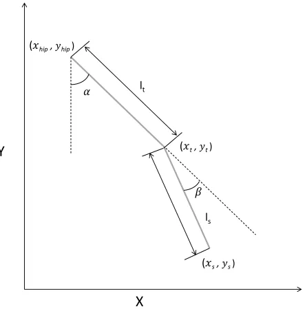
The forces and torques experienced by a leg in everyday conditions are primarily restricted to the saggital plane. The effects on the leg outside this plane are negligible. Thus, this model only considers the motion of the leg in the saggital plane.
This system comprising the leg wearing ATP can be represented by a planar 2-link biped model. During the swing phase, the foot can be simplified into a point. The shank segment can be considered to be an ATP. The length of thigh (lt) and shank (ls) are considered to
be known, since these can be measured very easily. The thigh and shank segments are also assumed to be Euler-Bernoulli beams of uniform densities. This does not introduce a significant error since the inertias of both segments are set independently in a reference range. This biped model has been depicted in Fig. 2.4.
2.2.2
Problem Formulation
The swing phase of gait has been modeled using Lagrangian Dynamics. Lagrange’s Equation can be expressed as follows
-d dt
∂T ∂q˙h
− ∂T
∂qh
=Qh, h=1, 2,· · ·,k (2.2)
where,T =kinetic energy of leg
qh=generalized coordinate
Qh=generalized force
2.2. GAIT MODELING CHAPTER 2. FUNDAMENTALS OF ATP
X Y
𝛼
𝛽
(𝑥hip, 𝑦hip )
(𝑥t, 𝑦t )
(𝑥s, 𝑦s )
lt
ls
Figure 2.4Biped Model
For the gait model, the Kinetic Energy is composed of
-T = (Total Kinetic Energy)hip+ (Total Kinetic Energy)knee
2.2. GAIT MODELING CHAPTER 2. FUNDAMENTALS OF ATP
And the Generalized force can be represented as
-Qh=
∂ ∂qh
Total Work Done by system
= ∂
∂qh
Workhip+Workknee
= ∂
∂qh
(Rotational Work+Work against gravity)hip+(Rotational Work+Work against gravity)knee
(2.4)
The generalized coordinates for the biped model are
-q = (α,β,xhip,yhip) (2.5)
where,α=hip angle
β=knee angle
xhip,yhip=horizontal and vertical position of hip
2.2.3
ODE Gait Model
The mathematical expressions are derived for Eq. 2.3 and Eq. 2.4. These expressions are then substituted in Eq. 2.2 and differentiated with respect to the generalized coordinates described in Eq. 2.5. This gives the set of four differential equations that describe the dynamics of the system about(α,β,xhip,yhip).
However, the equations corresponding toxhip,yhipare only useful if the hip position
2.2. GAIT MODELING CHAPTER 2. FUNDAMENTALS OF ATP
joint angles. These two equations are now presented.
Torque Equation 1, TE1
Ja +Jb +
1 3msl
2
s +mslsltcos β(t)
+mslt2+
1 3mtl
2
t
¨
α(t)
−
Jb +
1 3msl
2
s +
1
2mslsltcos β(t)
¨
β(t)
+1
2mslscos α(t)−β(t)
+msltcos(α(t)) +
1
2mtltcos(α(t))
¨
xhip(t)
+1
2mslssin α(t)−β(t)
+msltsin(α(t)) +
1
2mtltsin(α(t))
¨
yhip(t)
−mslsltsinβ(t)
˙
α(t)β˙(t) +1
2mslsltsin β(t)
˙
β(t)2
−1
2mslsg sinα(t)−β(t)
−msltgsin(α(t))−
1
2mtltgsin(α(t)) −τknee(t)−τhip(t) =0
(2.6)
Torque Equation 2, TE2
−
Jb +
1 3msl
2
s +
1
2mslsltcos β(t)
¨
α(t) +
Jb +
1 3msl
2
s
¨
β(t)
−1
2mslscos α(t)−β(t)
¨
xhip(t) −
1
2mslssinα(t)−β(t)
¨
yhip(t)
+1
2mslsltsinβ(t)
˙
α(t)2 +1
2mslsgsinα(t)−β(t)
+τknee(t) =0
CHAPTER
3
PHASE 1 - PARAMETER ESTIMATION
3.1. MOTIVATIONS AND OBJECTIVES CHAPTER 3. PARAMETER ESTIMATION
adopted. The chapter is summed up by a discussion of the results of this phase and future work that could help improve the results.
3.1
Motivations and Objectives
One of the requirements for effectively implementing a Model Predictive Controller is that a fairly accurate mathematical model of the system is needed, and a close approximation of all the system parameters involved is essential. Without a good approximation of the model or it’s parameters, the results produced by the Model Predictive Controller can be way off the mark from the desired results. In fact, such a controller can destabilize the system quickly, depending on how inaccurate our estimates are.
The Thigh-Knee-Shank Model describing the human gait, henceforth referred to as theSystem ModelorTKS Model, has four parameters which are directly dependent on the amputee wearing the prosthesis, who is henceforth referred to as thesubject. Namely, Thigh Mass(mt ),Shank Mass(ms ),Thigh Inertia(Ja ) andShank Inertia(Jb ). These four
parameters are collectively referred to as theinertial parameters.
These parameters are inherent to the system and a good estimate is essential before we can start designing a MPC based controller. However, as is apparent, it is not possible to directly measure these parameters. Neither is it possible to determine these parameters from some simple calculations based on data of the physical process. Estimation of these inertial parameters is the primary motivation behind this stage of the research.
3.2. OVERVIEW CHAPTER 3. PARAMETER ESTIMATION
fact the control system designer has freedom to choose these parameters depending on the desired performance characteristics. The aforementioned control technique has been used for collecting the data which will be used for estimating the system parameters. Thus, the problem of parameter estimation also involves estimating these control parame-ters. This provides us with a few extra degrees of freedom while determining estimates for the inertial parameters. However, it is desirable to have an estimate of the actual values of these parameters which were used for collecting the data. Success in getting control parameter estimates close to the originally used values would provide added confidence about the validity of the inertial parameter estimates.
3.2
Overview
The problem of estimating the system parameters has been treated as an optimization problem with the goal of fitting the calculated values of gait phase to measured data as best as possible. Before diving into the details of the optimization problem, it is beneficial to provide a high-level overview of the approach and present a brief discussion of the primary considerations behind the chosen approach. The inertial and control parameters to be estimated are treated as the optimization parameters. The nonlinear differential equations representing the system dynamics are used to calculate the gait phase values for the entire gait cycle. The deviation of these calculated parameter values from the measured parameter values is measured and this deviation is attempted to be minimized. Ideally, these deviations should be reduced to very small values as the parameter estimates reach a region very close to the actual values.
actua-3.2. OVERVIEW CHAPTER 3. PARAMETER ESTIMATION
tors might have unmodeled nonlinearities, which is easily possible in relatively inexpensive actuators. As a result, the actual torque produced by the actuators may not follow the de-sired control law very closely. Secondly, quantitative information regarding the interaction of the leg with the hip and upper body might be unavailable. The effects of these and some other factors influencing the results will be discussed in greater detail in later sections. However, as can be seen already, these factors make it practically impossible to follow the measured data very accurately. So it can be tough to determine when we have reached the minima of this optimization problem. The problem is further complicated by the existence of many local minima since the design space is highly non-convex.
3.3. PROBLEM FORMULATION CHAPTER 3. PARAMETER ESTIMATION
3.3
Problem Formulation
As discussed in previous section, this optimization problem needs to be broken down into smaller steps such that the individual problems are of a manageable size for the opti-mization algorithms. At each of the steps in the optiopti-mization process, a hybrid algorithm composed of aglobalandlocalsolver are used, unless otherwise noted. This hybrid algo-rithm makes it possible to quickly search over large regions of the design space using a
global solverand identify regions which could potentially provide good solutions. Once a few good regions are identified, the optimization is then handed over to alocal solver
which can then quickly identify the best solutions within these regions. The optimization process is agnostic to the actual global and local solvers used at every step.
Two different optimization strategies were examined for this problem, and then a com-bination of the two was finally implemented such that the strengths of both the strategies are combined. The following sections and subsections explain some common terminology used henceforth, followed by an explanation of the two major strategies used and their respective advantages and disadvantages. The final optimization process is then presented followed by the actual local and global optimization solvers, and other implementation details.
3.3.1
Terminology Used
3.3. PROBLEM FORMULATION CHAPTER 3. PARAMETER ESTIMATION
and process and are essential to understanding the material that follows. Hence, it would be appropriate to discuss the terminology used in advance.
Subject Parameters
Subject Parameterscollectively refers to the set of parameters which are either inherent to the subject or are defined during the control design process. These parameters remain constant during the entire gait cycle. They can be further subdivided as follows
-1. Inertial Parameters
-These parameters are inherent to the subject and are the primary goal of this phase of the research.
• mt - Mass of the thigh segment of the amputee, as defined by Dempster Body
Segment Data[Win09]. However, as described previously, a healthy subject was used for collecting the data while wearing a prosthetic adapter. Hence, for this research,mt will actually be the mass of the entire lower limb. For future work,
if data collection is done for an amputee subject, this parameter should be used as originally defined.
• ms - Mass of the shank segment of the amputee, as defined by Dempster Body
Segment Data[Win09].
• Ja - Mass moment of Inertia of the thigh segment.
• Jb - Mass moment of Inertia of the shank segment.
2. Control Parameters
3.3. PROBLEM FORMULATION CHAPTER 3. PARAMETER ESTIMATION
the freedom to choose these parameters such that the system meets the performance requirements. Even though they are not the primary goal for this phase of the research, including them as optimization parameters provides extra degrees of freedom. Also, getting a good approximation of these values, as compared to the actual values used, provides reaffirmation regarding the validity of the inertial parameter estimates.
• Kflex,Kext- Proportional gain for the knee angle, for flexion and extension cycle
respectively.
• dflex,dext- Proportional gain for the knee angular velocity, for flexion and
exten-sion cycle respectively.
• ¯βflex, ¯βext- Reference knee angle, for flexion and extension cycle respectively.
Cycle Kinematic Parameters
Cycle Kinematic Parameterscollectively refers to the states of the system and their deriva-tives. Thus, values for these parameters are time dependent and are stored separately for all the time steps in the gait cycle. They can be further subdivided as follows
-1. Knee Angular Parameters
-• β- Knee Angle
• ˙β- Knee Angular Velocity • ¨β- Knee Angular Acceleration
2. Hip Angular Parameters
3.3. PROBLEM FORMULATION CHAPTER 3. PARAMETER ESTIMATION
• ˙α- Hip Angular Velocity • ¨α- Hip Angular Acceleration
3. Hip Coordinate Parameters
-• x - Hip Horizontal Position • ˙x - Hip Horizontal Velocity • ¨x - Hip Horizontal Acceleration • y - Hip Vertical Position
• ˙y - Hip Vertical Velocity • ¨y - Hip Vertical Acceleration
Evaluated Parameters
Evaluated Parameterscollectively refers to the parameters that are not known at the outset and are determined from the gait data by performing some calculations. These parameters are
-• Ceq- A vector containing the constraint violations for all the equality constraints of
the optimization problem.
• τknee- The torque applied at the knee by the actuator of the prosthetic leg.
• τhip- The torque applied by the subject at the hip joint.
3.3.2
Optimization Parameters
3.3. PROBLEM FORMULATION CHAPTER 3. PARAMETER ESTIMATION
Design Parameters. Which of the previously described parameters are used as optimization parameters varies with the strategy being used and will be explained separately for each strategy. They are represented as
-di=ithoptimization parameter,∀i =1 ton
where,n=number of optimization parameters
Designrefers to any combination of values for the optimization parameters that is being evaluated as a possible solution to the optimization problem. The order of the optimization parameters within a design is irrelevant. When the design is expressed in vector form, it is also referred to as theDesign Vectorand can be represented as
-D = [d1, . . . ,dn] (3.1)
3.3.3
Constraints
Constraint Equationsrefers to the nonlinear differential equations which need to be satis-fied by any design in order to be considered a feasible solution. As explained previously, only the torque equations from the system model will be used for this phase of the research. They are referred to as
-• TE1- Refers to Eq. 2.6. This equation is used for calculatingαand it’s derivatives. • TE2- Refers to Eq. 2.7. This equation is used for calculatingβand it’s derivatives.
3.3. PROBLEM FORMULATION CHAPTER 3. PARAMETER ESTIMATION
3.3.4
Weighted Parameters
Weighted Parameterscollectively refers to the set of parameters whose deviations are measured and weighted in the cost function. They are independent of the optimization parameters, since deviations are only relevant for cycle parameters. Explicitly specifying weighted parameters also provides the flexibility of including only some of the cycle pa-rameters. Whereas, optimization parameters may include some or all of subject and cycle parameters. The set of weighted parameters can be represented as
-Ω= [ω1, . . . ,ωm], (3.2)
where,m= number of weighted parameters
and,ωi= variable representing any generic system parameter
Each weighted parameter needs to be assigned a numerical weight. The absolute mag-nitude of these variables is not significant. But their magmag-nitude relative to each other represents the degree to which their accurate matching is important. The weights can be represented in vector form as follows
-W = [w1, . . . ,wm] (3.3)
3.3. PROBLEM FORMULATION CHAPTER 3. PARAMETER ESTIMATION
3.3.5
Cost Function
The objective of the optimization problem is to find a design that minimizes the cost func-tion. The cost function value is evaluated for every design with a lower value representing a better design. Since the goal of the optimization is to fit the calculated data to the mea-sured data as best as possible, the cost function is defined such that it returns the weighted squared deviation of the calculated data. However, the individual parameter deviations need to be normalized with respect to its maximum measured value. This ensures that the difference in scale of the individual parameters doesn’t skew the cost function value. The cost function can be expressed as follows
-J =
m
X
i=1
wi·(bxi−x¯i)
2
max|x¯i|
(3.4)
where,bxi=vector containing calculated value ofωi for entire gait cycle ¯
xi=vector containing measured value ofωi for entire gait cycle max|x¯i|=maximum absolute value ofithparameter from measurements
and, both are vectors containing the parameter value for all time steps
Although it should be noted that there isn’t enough quantitative information available re-garding theτhipprofile during the gait cycle. Existing studies mostly focus on the qualitative nature of howτhipvaries over the cycle and its interplay with other factors. There were certainly noτhipmeasurements available for this study. However, analysis of gait data for
indi-3.4. OPTIMIZATION STRATEGIES CHAPTER 3. PARAMETER ESTIMATION
cates that having lower magnitude ofτhipmight be more energetically efficient. And even though the magnitude ofτhipfor amputees might turn out to be higher as compared toτknee
for amputees, it is desirable to minimizeτhipas much as possible. For this reason, whenever
τhipis to be included as a weighted parameter, instead of measuring the deviations from
some measured value, its norm will be penalized. However, the corresponding weight will be maintained at a relatively low value, since accurately tracking hip and knee parameters is of greater concern.
3.4
Optimization Strategies
As described previously, the following two distinct optimization strategies were adopted for the purpose of this research
-1. Differential Equation Solver Method 2. Discrete Optimization Method
3.4. OPTIMIZATION STRATEGIES CHAPTER 3. PARAMETER ESTIMATION
3.4.1
Differential Equation Solver Method
TheOptimization Parametersfor this method are chosen from the set of subject parameters. When the inertias of thigh or shank are included as Optimization Parameters, their values are set independently of the mass values of the respective segments, albeit in a range that is still linked to the respective mass values. If these parameters are not included however, their values are coupled to the respective mass values using the following relation
-ja=ktmtlt2 jb =ksmsls2 (3.5)
where,ktandksare the radii of gyration of the thigh and shank segments respectively, and
their values are obtained from statistical models presented in[Win09].
The solver generates new designs by picking values for the chosen optimization param-eters within the specified range. And as the name suggests, the nonlinear state equations are then solved over the entire gait cycle in order to generate values for the state variables, which we refer to as cycle parameters, for all time steps. This calculated data is then used to evaluate the design based on the cost function value. The major advantage offered by this method is that it eliminates the need for satisfying nonlinear constraints at all time steps. This reduces the computational burden significantly and provides the ability to quickly scan large areas of the design space.
3.4. OPTIMIZATION STRATEGIES CHAPTER 3. PARAMETER ESTIMATION
3.4.1.1 Optimizing with coupled State Equations
As the name suggests, this method uses the coupled system of differential equations to solve for all cycle parameters.α,β and their first derivatives are treated as the state variables. The measured data is only used for setting the initial conditions. After that, the derivative values obtained from the system of state equations (TE1and TE2) are used for updating the values of state variables at each time step. Since all the cycle parameters are being solved for, all their deviations needs to be measured in addition toτhip, which is treated as an
independent optimization parameter. However, depending on the priority, the magnitude of these weights can be adjusted such that greater emphasis is placed on matching some of these parameters instead of trying to match all of them equally.
Intuitively, this method seems a very elegant way of solving the optimization problem since it combines all the cycle parameters into one problem without having to satisfy nonlinear constraints at all time steps. However, this method presents many challenges. Firstly,τhipbeing an independent optimization parameter needs to be estimated at all time steps in the gait cycle such that it satisfies TE1. And since all the other cycle parameters are
not being controlled independently at all time steps, it is incredibly tough to get a good estimate forτhipwithout having a closed-form solution, or at least a reference curve to track.
3.4. OPTIMIZATION STRATEGIES CHAPTER 3. PARAMETER ESTIMATION
variables, and provide misleading indications about the direction that some parameters need to take. This problem can be tackled by decoupling the state equations, and as a result, the state variables. The decoupled state equations can then be used to solve different aspects of the problem.
3.4.1.2 Optimizing with TE2only
This method only uses TE2to solve for (β, ˙β , ¨β). Measured values of (α, ˙α, ¨α) are used at all time steps for performing the required calculations. TE1is used to calculate the value of
τhipat all time steps that would perfectly satisfy the equation.
Since,αand its derivatives are not being calculated, there is no need to measure their deviations from the measured values. Although, as explained in subsection 3.3.5, it is required to minimizeτhipas much as possible. Thus, the weighted parameters includeβ ,
˙
β, ¨βandτhip. This method separates the problem of estimating the subject parameters for
optimal tracking ofβand its derivatives, which is the more important goal for this problem.
3.4.1.3 Optimizing with TE1only
Similar to the method described in subsubsection 3.4.1.2, this method only uses TE1 .
However, TE1contains an additional unknown variable in the form ofτhip. Thus, unlike the previous method, this can not be used to solve for (α, ˙α, ¨α). Instead, measured values of all cycle parameters are used to solve forτhipwhich would satisfy the equation perfectly.
Since none of the cycle parameters are being calculated, there is no need to measure their deviations from the measured values. Instead the norm ofτhipis the sole quantity
3.4. OPTIMIZATION STRATEGIES CHAPTER 3. PARAMETER ESTIMATION
the subject parameters for minimizing theτhipthat a subject needs to apply during the gait cycle, thus minimizing the energy spent by the subject.
3.4.2
Discrete Optimization Method
TheOptimization Parametersfor this method include a combination of subject parameters, and some or all of cycle parameters. The inertias of the thigh and shank segments can be independent or coupled to respective masses, as described in subsection 3.4.1.
For every design, the solver generates a value for each subject parameter in their spec-ified ranges. Similarly, it generates a value for all cycle parameters included in the set of optimization parameters, at each time step. Generally, only one out ofα(β) and its deriva-tives is chosen, and the other derivaderiva-tives are calculated using finite difference method. These cycle parameters are subject to constraints which limit the maximum change in any given parameter between successive time steps. The design is also required to satisfy the nonlinear constraints (TE1and/or TE2, depending on variation) at each time step. And
measured values are used for all cycle parameters that are not included as optimization parameters.
3.4. OPTIMIZATION STRATEGIES CHAPTER 3. PARAMETER ESTIMATION
judiciously.
As withDE Solver Method, this method also has its own variations which are now dis-cussed in detail.
3.4.2.1 Optimizing with coupled State Equations
This method presents the most obvious variation of the method explained above. Opti-mization Parametersinclude bothαandβ , in addition to the subject parameters. The design needs to satisfy TE1as well as TE2at every time step. And since both sets of cycle parameters are being optimized, both of them need to be weighted as well. Whetherτhipis
penalized in the cost function depends on the method chosen for handling it.
Although this method is the most broadly applicable, it also carries with it the most amount of computational burden. And the sheer number of optimization parameters mean that it is not feasible to get any meaningful results using this method directly. However once a decent estimate is available for the design, this method can prove to be handy while trying to refine the estimate. As was the case with subsection 3.4.1, the methods described next will help in overcoming some of these difficulties.
3.4.2.2 Optimizing with TE2only
For every design generated by the solver, this method only imposes TE2as the nonlinear equality constraint, in addition to the linear inequality constraint previously described. Besides the subject parameters,Optimization Parametersmay include any combination of
α,β and their derivatives. And since cycle parameters are independently determined at
3.5. OPTIMIZATION ROADMAP CHAPTER 3. PARAMETER ESTIMATION
This was not possible with theDE Solver Methodsince the state equations corresponding to
x andy are not being considered due to lack of knowledge regarding hip forces. Measured values are used for whichever cycle parameter is not included as an optimization parameter.
3.4.2.3 Optimizing with TE1only
This method is very similar to subsubsection 3.4.2.2. It imposes TE2as the nonlinear equality
constraint instead of TE1. However, it does have an extra parameter in the form ofτhip.
There are two different ways for handlingτhipthough. Like the other cycle parameters,
τhipcan be treated as an independent optimization parameter, and estimated at each time
step such that it satisfies the constraints as closely as possible. Alternatively,τhipcan be determined by solving for it’s value at each time step from TE1based on the values deter-mined for other cycle parameters by the solver. When this method is used for determining
τhip, it needs to be included as a weighted parameter in the cost function. Otherwise,τhip
would absorb all the error in the equation and would return a cost function value of zero for any design. In the absence of a reference curve forτhip, this method is much more effective,
direct and computationally efficient. In fact, keepingαandβ constant and solving solely forτhipcan be used as a quick way to explore the design space of the subject parameters.
3.5
Optimization Roadmap
3.5. OPTIMIZATION ROADMAP CHAPTER 3. PARAMETER ESTIMATION
at different stages. Further, it turns out that the dynamics of the extension phase of the gait cycle are much more complicated and tougher to satisfy as compared to the flexion phase. Thus, estimating parameters for flexion phase is much easier. The result is an elaborate procedure with many steps along the way such that the different subject parameters are estimated sequentially and their estimates refined gradually, instead of trying to estimate all of them at once.
Estimating Parameters for Flexion Phase
For this phase of the optimization process, only data corresponding to the flexion phase is used. Thus, the relevant subject parameters only include theinertial parametersand
flexion control parameters.
(a) Use DE Solver Method with TE2only
-This step yields a decent estimate forms andJb . Also, it helps to evaluate the design
space for flexion control parameters (Kflex,dflex, ¯βflex) and determine which regions
could provide promising results.
(b) Use Discrete Optimization Method with TE2only
-Since decent estimates are already available forms and Jb , this step helps to further
refine these estimates. This should result in an approximation that is pretty close to the real values of these parameters. This step also serves to narrow down the regions for flexion control parameters. But these estimates are still relatively rough and leave room for improvement.
-3.5. OPTIMIZATION ROADMAP CHAPTER 3. PARAMETER ESTIMATION
The values forms , Jb and flexion control parameters are fixed to the center of their
estimated ranges for now. The system performance is now evaluated by varyingms
andJa over relatively wide ranges in order to try and minimizeτhipto estimate the
regions in design space that would yield promising results forms and Ja .
(d) Use Discrete Optimization Method with TE1only
-This step serves to fine-tune the estimates of flexion control parameters. It also helps to narrow down the range formt andJa , but these estimates are still relatively rough
and will be improved upon later.
(e) Use Discrete Optimization Method with coupled State Equations
-Now that estimates forms , Jb and the flexion control parameters have been
consider-ably fine-tuned, onlymt and Ja still remain with rough estimates. This is the perfect
type of scenario for exploiting the strengths of this method. Thus all subject parame-ters (inertial and control), along with cycle parameparame-ters, are included as optimization parameters and the estimates ofmt and Ja are refined.
By this point in the optimization process, the estimates obtained for the inertial parameters and flexion control parameters should be in fairly nnarrow regions around the actual values. Using this knowledge, estimation of extension control parameters can now be performed.
Estimating Parameters for Extension Phase
For this phase of the optimization process, only data corresponding to the extension phase is used. Thus, the relevant subject parameters only include theinertial parametersand
3.6. IMPLEMENTATION DETAILS CHAPTER 3. PARAMETER ESTIMATION
(a) Use DE Solver Method with TE1only
-All the inertial parameters are fixed to the center of their respective range, which should be very narrow now. Similar to flexion cycle, the system performance is now evaluated by varying extension control parameters over relatively wide ranges and attempting to minimizeτhip. This helps to estimate the regions in design space which
would provide promising results for the extension control parameters
(b) Use Discrete Optimization Method with TE1only
-This step serves to narrow down estimates of extension control parameters.
(c) Use Discrete Optimization Method with coupled State Equations
-As with flexion cycle, the last step is to solve for the coupled state equations while including all subject parameters as optimization parameters. However there is a small difference here. It turns out that it is really tough to get a good fit for TE2for a variety of reasons which will be discussed later. Thus,βis not included in optimization parameters, whereasαis. The method then tries to refine the estimates by minimizing
τhipfor TE1and the constraint violation for TE2.
Thus, by breaking the problem down into multiple steps, all the subject parameters can be estimated with reasonable accuracy.
3.6
Optimization Solver - Implementation Details
3.6. IMPLEMENTATION DETAILS CHAPTER 3. PARAMETER ESTIMATION
to certain principles. This section examines some of the considerations while choosing a solver and tuning its parameters.
3.6.1
Choice of Solver
As explained previously in section 3.2, the strengths of aglobalandlocaloptimization solver can be combined by using ahybridscheme. Such a hybrid scheme would use a global solver initially to scan large regions of the design space and identify regions which could provide promising designs. It would then hand over the optimization in these regions to a local solver which can efficiently and accurately determine the solutions in these regions. The choice then boils down to choosing a global and a local solver to be a part of this hybrid solver.
3.6. IMPLEMENTATION DETAILS CHAPTER 3. PARAMETER ESTIMATION
found here[Mat16a]. Instead the forthcoming sections will focus on how this solver is adapted for the needs of the problem at hand. When used in conjunction with the MATLAB Parallel Computing Toolbox[Mat16j], lot of the computations at each generation can be parallelized. This results in huge gains in efficiency and reduces the computational time by a large margin.
The MATLAB Optimization Toolbox[Mat16i]provides a wide variety of options of local solvers as well. As explained by[Mat16h], the best option for nonlinear constrained op-timization problem isfmincon. It essentially provides an implementation of the interior point algorithm as described in[Wik16]. An elaborate explanation of the working offmincon has been provided in[Mat16c].
3.6.2
Initial Estimate
Genetic algorithm can find an optimal, or nearly optimal solution, regardless of the initial estimate. Nevertheless, providing a good initial estimate can be of huge benefit in a highly non-convex problem like this.
[Win09]provides body segment parameter data for 2D studies collected from statistical
3.6. IMPLEMENTATION DETAILS CHAPTER 3. PARAMETER ESTIMATION
starting estimate, and definitely better than any initial estimate that can obtained from another source.
For control parameters, one needs to rely on the estimate provided by the researchers performing the data collection experiments. These estimates can come with caveats of their own. Depending on the type of equipment used for control of the prosthesis, precise values of these control parameters may not be available to these researchers themselves. Additionally, depending on the quality and nature of actuation devices, it may not be able to follow the desired control law accurately, as explained in section 3.2. Thus, greater flexibility can be allowed in the estimation of these control parameters as long as their estimates lie in similar regions.
3.6.3
Parameter Weights
3.6. IMPLEMENTATION DETAILS CHAPTER 3. PARAMETER ESTIMATION
in the following form where x represents any generic cycle parameter
-x
˙
x ∝
1 ∆t
where,∆t =sampling time for measured data
The deviations of the calculated parameters from measured parameters should be nor-malized with respect to the maximum measured value of that parameter. Otherwise, the difference in scale of the various parameters would unfairly skew the quantities being penalized in the cost function and would thus have the undesirable effect of shifting the emphasis of optimization.
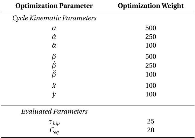
Table 3.1Reference Values for Optimization Parameter Weights
Optimization Parameter Optimization Weight
Cycle Kinematic Parameters
α 500
˙
α 250
¨
α 100
β 500
˙
β 250
¨
β 100
¨
x 100
¨
y 100
Evaluated Parameters
τhip 25
3.6. IMPLEMENTATION DETAILS CHAPTER 3. PARAMETER ESTIMATION
It should be noted that since no reference measurements are available forτhip , the calculated values of this parameter can not be normalized. Thus, the weight forτhipneeds
to be manually calibrated taking into account its magnitude.
There is no unique value of the parameter weights that return the best results and a lot of freedom is available for choosing their exact values. They need to be determined individually for the different steps in the optimization roadmap by trial. Nevertheless, some guidance regarding their relative magnitudes and ranges can prove to be useful. Values provided in Table 3.1 can be used for reference.
3.6.4
Additional Adaptations for Speed
As mentioned several times, this optimization process is very computationally intensive. Even after parallelizing the computations on a local machine, one optimization run can easily take several days to complete in order to get any meaningful results. This is clearly not a desirable scenario. It would take up valuable computing resources on a local machine and make it very tough to try out new variations of existing strategies.
3.7. DISCUSSION OF RESULTS CHAPTER 3. PARAMETER ESTIMATION
The High Performance Computing Cluster of NC State University[Uni16]was used for the purpose of this research.
3.7
Discussion of Results
The final estimates obtained for theSubject Parametersare now presented along with a visualization of the output of the simulated gait cycle. This will be followed by a discussion of the possible factors affecting the results and the factors that could help to improve these results.
3.7.1
Subject Parameter Estimates
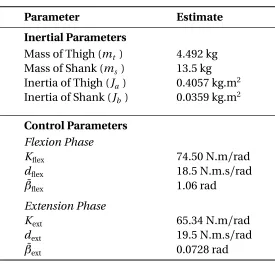
The final estimates of the subject parameters that returned the best possible match for the hip and knee angles are listed in Table 3.2.
The important parameters to note here are theInertial Parameters. Estimating these was the primary goal of this phase of the research, since their knowledge is essential for designing a Model Predictive Controller. The values ofControl Parametersare essential for getting a good estimate of the knee torques and thus satisfying the nonlinear constraints. However, they are not essential for the control design process.
The accuracy of these estimates will now be analyzed.
3.7.2
Analysis of Results
3.7. DISCUSSION OF RESULTS CHAPTER 3. PARAMETER ESTIMATION
Table 3.2Final estimates of Subject Parameters
Parameter Estimate
Inertial Parameters
Mass of Thigh (mt ) 4.492 kg
Mass of Shank (ms ) 13.5 kg
Inertia of Thigh (Ja ) 0.4057 kg.m2
Inertia of Shank (Jb ) 0.0359 kg.m2
Control Parameters
Flexion Phase
Kflex 74.50 N.m/rad
dflex 18.5 N.m.s/rad
¯
βflex 1.06 rad
Extension Phase
Kext 65.34 N.m/rad
dext 19.5 N.m.s/rad
¯
βext 0.0728 rad
is a high degree of coupling present between TE1and TE2. Any small error in calculation of ¨
αin TE1manifests itself in TE2leading to an error in ¨β as well. The converse of this is also
true, with an error in ¨β leading to an error in ¨α. Thus, the error cascades into a very large value in short amount of time, and it becomes tough to isolate the cause of the error. It can also give misleading indications about the degree of inaccuracy of the parameter estimates.
To overcome this problem, and to be able to gauge the accuracy of estimates, the decoupled state equations are solved instead. In order to visualize the matching ofα, only TE1is solved over time usingαand its derivatives as the state variables. The measured values ofβ and its derivatives are used in this equation. Theτhipvalues required to satisfy
3.7. DISCUSSION OF RESULTS CHAPTER 3. PARAMETER ESTIMATION
Similarly, to visualize the matching ofβ , only TE2is solved over time usingβ and its derivatives as the state variables. The measured values ofαand its derivatives are used in this equation. Theτkneevalues required to satisfy this equation are also calculated and
plotted. Estimates ofτhipandτknee can not be compared to their actual values since no
measurements are available for them. Nevertheless, these estimates will prove useful in order to compare the performance of the controller in the next phase of the research.
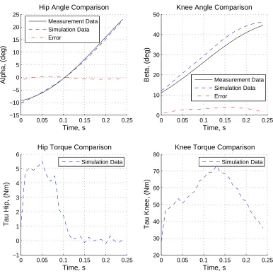
Flexion Phase
The method explained above was used for visualizing the accuracy of the estimated param-eters for the flexion phase and the results are presented in Fig. 3.1. It should be noted that the scales used for plottingαandβ are different. Similarly, the scales forτhipandτkneeare
different. This is done because forcing the quantities to be plotted on the same scale would not allow their variation to be visualized properly. As can be observed from the plots, the values ofαandβare matched with very high accuracy and providing confidence about the accuracy of these estimates.
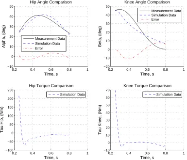
Extension Phase
The accuracy of estimated parameters for extension phase was visualized similarly, and has been presented in Fig. 3.2. It can be observed that the matching of parameters is not as good as it was in the flexion phase. However, this is to be expected since the dynamics of extension phase are much more complex as compared to the flexion phase, and the matching of joint angles can be considered reasonable.
3.7. DISCUSSION OF RESULTS CHAPTER 3. PARAMETER ESTIMATION
0 0.05 0.1 0.15 0.2 0.25
−15 −10 −5 0 5 10 15 20 25 Time, s Alpha, (deg)
Hip Angle Comparison
Measurement Data Simulation Data Error
0 0.05 0.1 0.15 0.2 0.25
0 10 20 30 40 50 Time, s Beta, (deg)
Knee Angle Comparison
Measurement Data Simulation Data Error
0 0.05 0.1 0.15 0.2 0.25
−1 0 1 2 3 4 5 6 Time, s
Tau Hip, (Nm)
Hip Torque Comparison
Simulation Data
0 0.05 0.1 0.15 0.2 0.25
20 30 40 50 60 70 80 Time, s
Tau Knee, (Nm)
Knee Torque Comparison
Simulation Data
3.7. DISCUSSION OF RESULTS CHAPTER 3. PARAMETER ESTIMATION
spike in values of bothτhipandτkneeat the start of the cycle. This can be understood by observing the rate of change ofβ . Simulated value ofβ starts decreasing at a greater rate as compared to the measured value. Since the control law forτkneeis linearly dependent on
˙
β , this results in a greater value ofτknee. This in turn leads to an increase inτhip, in order
to compensate for the error produced in TE1.
Another possible reason of concern is the higher value ofτhip than that observed in healthy individuals. Although this may seem to be a limitation of this result, it is in fact a logical outcome. Studies[LF08]have shown that there exists a strong interplay between the hip torque and ankle push-off. A higher ankle push-off at the start of the swing phase provides greater momentum to the leg, which carries it through the swing phase and thus requires a reduced effort at the hip. Whenever there is a reduction in ankle push-off due to physical injury, some medical condition, or with progression of age, humans automatically compensate for it by increasing the hip torque. Since the prototype used for data collection did not have an actuated ankle joint, there was no ankle push-off available. Thus, there is no initial momentum available and the hip joint has to perform greater amount of work to
pullthe leg through.
Future studies that measure the applied hip torque can help to test the validity of this hypothesis. Performing data collection using a prosthesis with an actuated ankle joint can also help in this regard.
3.7. DISCUSSION OF RESULTS CHAPTER 3. PARAMETER ESTIMATION
0.2 0.4 0.6 0.8 1 −10 0 10 20 30 40 50 Time, s Alpha, (deg)
Hip Angle Comparison
Measurement Data Simulation Data Error
0.2 0.4 0.6 0.8 1 −20 −10 0 10 20 30 40 50 Time, s Beta, (deg)
Knee Angle Comparison
Measurement Data Simulation Data Error
0.2 0.4 0.6 0.8 1 −100 −50 0 50 100 150 200 250 Time, s
Tau Hip, (Nm)
Hip Torque Comparison
Simulation Data
0.2 0.4 0.6 0.8 1 −10 0 10 20 30 40 50 60 70 Time, s
Tau Knee, (Nm)
Knee Torque Comparison
Simulation Data
3.7. DISCUSSION OF RESULTS CHAPTER 3. PARAMETER ESTIMATION

![Figure 4.2 Basic concept of Model Predictive Control. Adapted from [Seb11]](https://thumb-us.123doks.com/thumbv2/123dok_us/1474298.1180532/72.612.145.497.310.543/figure-basic-concept-model-predictive-control-adapted-seb.webp)
