Dissertations
2013
Estimating multiple treatment effects in two-phase
observational data
Bin Liu
Iowa State University
Follow this and additional works at:https://lib.dr.iastate.edu/etd
Part of theStatistics and Probability Commons
This Dissertation is brought to you for free and open access by the Iowa State University Capstones, Theses and Dissertations at Iowa State University Digital Repository. It has been accepted for inclusion in Graduate Theses and Dissertations by an authorized administrator of Iowa State University Digital Repository. For more information, please [email protected].
Recommended Citation
Liu, Bin, "Estimating multiple treatment effects in two-phase observational data" (2013).Graduate Theses and Dissertations. 13505.
by
Bin Liu
A dissertation submitted to the graduate faculty in partial fulfillment of the requirements for the degree of
DOCTOR OF PHILOSOPHY
Major: Statistics
Program of Study Committee: Cindy Yu, Major Professor
Alicia Carriquiry Kenneth J. Koehler
Sarah M. Nusser Huaiqing Wu
Iowa State University Ames, Iowa
2013
DEDICATION
I would like to dedicate this thesis to my parents and my brother and to my girlfriend Xiaoqing Zhou without whose support I would not have been able to complete this work. I would also like to thank my friends and family for their warm support during the writing of this work.
TABLE OF CONTENTS
LIST OF TABLES . . . v LIST OF FIGURES . . . vi ACKNOWLEDGEMENTS . . . vii ABSTRACT . . . viii CHAPTER 1. OVERVIEW . . . 1 1.1 Introduction . . . 1CHAPTER 2. ESTIMATING MULTIPLE TREATMENT EFFECTS USING TWO-PHASE REGRESSION ESTIMATORS . . . 6
2.1 Proposed Two-Phase Semiparametric Regression Estimators . . . 6
2.1.1 Basic Set-up and The Proposed Estimator . . . 7
2.1.2 Notations and Assumptions . . . 9
2.1.3 The Central Limit Theorem of θbg . . . 10
2.1.4 A Central Limit Theorem of bθ = [θb1,θb2, ...,θbG]T . . . 19
2.2 Simulation Study . . . 21
2.3 Conclusion and Remarks . . . 26
CHAPTER 3. ESTIMATING MULTIPLE TREATMENT EFFECTS USING GENERALIZED ESTIMATING EQUATIONS . . . 32
3.1 Introduction . . . 32
3.2 Basic Set Up and the Proposed GMM Estimator . . . 35
3.2.2 Assumptions . . . 38
3.2.3 Consistency and Normality Theorems . . . 39
3.2.4 A Variance Estimator . . . 41
3.3 The Empirical Likelihood Estimator . . . 43
3.3.1 Introduction . . . 43
3.3.2 Set-up and the Proposed EL Estimator . . . 44
3.3.3 Calculation Procedure for (ˆλT,θˆT EL)T and Estimated Variance . . 49
3.4 Simulations . . . 50
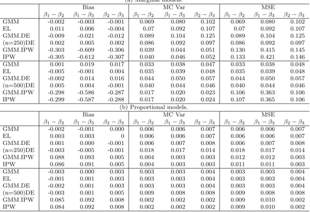
3.4.1 Marginal and Proportional Models . . . 52
3.5 Conclusion . . . 54
CHAPTER 4. REAL DATA STUDY . . . 59
4.1 Two-phase Regression Estimates . . . 60
4.2 The GMM Estimator and the EL Estimator: Difference in Means and Proportions . . . 62
CHAPTER 5. CONCLUSIONS AND FURTHER STUDIES . . . 66
APPENDIX PROOF OF THEOREMS . . . 68
LIST OF TABLES
Table 2.1 The MC biases, variances and MSEs of the estimated treatment
effects, for (1): (N, n) = (12500,250); (2): (N, n) = (25000,500); (3): (N, n) = (50000,1000). . . 28
Table 2.2 The coverage probabilities of the 95% C.I. for estimated treatment
effects, for (1): (N, n) = (12500,250); (2): (N, n) = (25000,500); (3): (N, n) = (50000,1000). . . 30
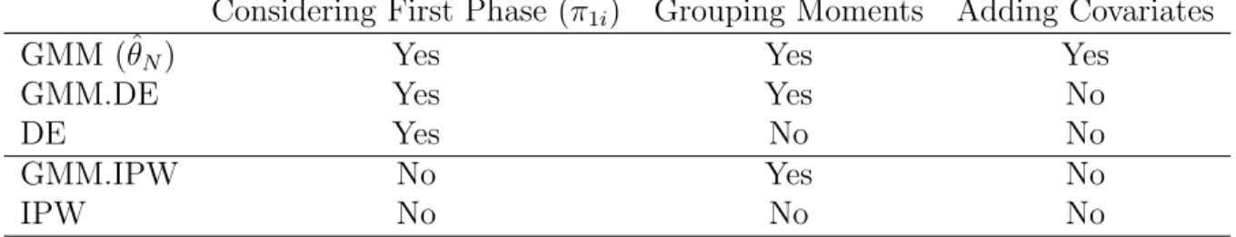
Table 3.1 Estimator comparisons . . . 54
Table 3.2 The MC biases, variances and MSEs of the estimated parameters
in marginal and proportional models. . . 57
Table 3.3 The coverage probabilities of the 95% C.I. for the proposed
esti-mator in marginal and proportional models. . . 58
Table 4.1 Results from the empirical study of nutrition label uses, including
estimated treatment effects for three nutrition label use levels, their standard errors and their 95% C.I.s. . . 61
Table 4.2 Marginal difference estimates . . . 63
LIST OF FIGURES
Figure 2.1 The plots of Monte Carlo averages (panel (a)) and root mean
square errors (panel (b)) of estimated treatment means versus
treatment levels in Example 1. . . 29
Figure 2.2 The plots of Monte Carlo averages (panel (a)) and root mean
square errors (panel (b)) of estimated treatment means versus
treatment levels in Example 2. . . 31
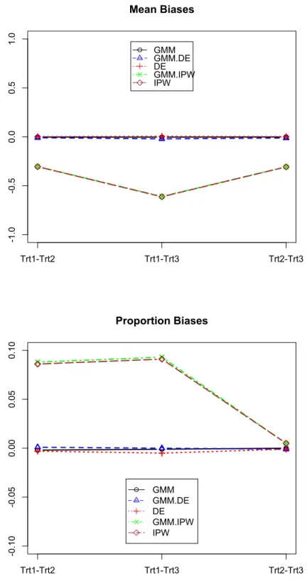
Figure 3.1 Monte Carlo averages of treatment difference bias in mean and
proportion models. (n = 250) . . . 55
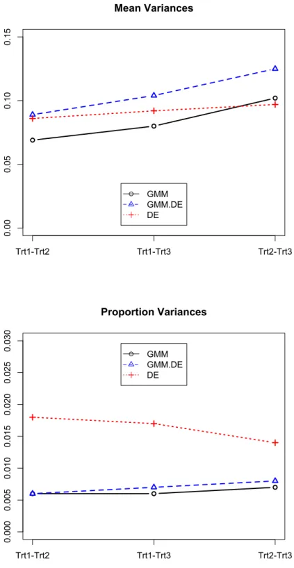
Figure 3.2 Monte Carlo variance of treatment difference in mean and
pro-portion models. (n = 250) . . . 56
Figure 4.1 The plot of estimated treatment means versus treatment levels in
ACKNOWLEDGEMENTS
I would like to take this opportunity to express my thanks to those who helped me with various aspects of conducting research and the writing of this thesis. First and foremost, Dr. Cindy Yu for her guidance, patience and support throughout this research and the writing of this thesis. Her insights and words of encouragement have often inspired me and renewed my hopes for completing my graduate education. I would also like to thank my committee members for their efforts and contributions to this work: Dr. Alicia Carriquiry, Dr. Kenneth J. Koehler, Dr. Sarah M. Nusser, and Dr. Huaiqing Wu. I would like to thank Dr. Carriquiry for her job hunting information, and Dr. Koehler and Dr. Nusser for their firm assistantship support, and Dr. Wu for his strong recommendation on job references. I would additionally like to thank Dr. Yu for her forever encouragement throughout the stages of my PhD research and job hunting. I would like to thank Dr. Jason Legg for bringing the research topic. Last, I would like to thank my friends Eunice Kim and Haley Nguyen for their special roles in my life.
ABSTRACT
We propose three estimators: Two-phase Regression (TPR), Generalized Method of Moments (GMM), and Empirical Likelihood (EL) estimators to estimate multiple treatment effects in two-phase observational data. They use semiparametric generalized propensity scores in estimating average treatment effects in the presence of informative first-phase sampling. The proposed estimators can be easily extended to any number of treatments and do not rely on a prespecified form of the treatment selection func-tions. All of the three proposed estimators have considered the first phase and second phase inclusion probabilities in their propensity scores to eliminate the biases resulted from ignoring survey sampling designs and selection bias. The proposed TPR estimator which deals with continuous response is shown to have improved efficiency compared to the double expansion estimators using sieve semiparametric regressions. The GMM and EL estimators, which estimate treatment effects defined through generalized estimating equations, reduce Monte Carlo variance by adding covariates and combing all the gen-eralized estimating equations in treatment groups. Results from simulation studies and real data studies for three estimators are presented.
CHAPTER 1.
OVERVIEW
1.1
Introduction
Timely comparative treatment analysis is useful for physician recommendations, pa-tient awareness, regulatory agency assessments of benefit-risk profiles, and
reimburse-ment agency cost effectiveness assessreimburse-ments. The use of observational data for such
purposes has grown significantly in number of studies and importance (Sorenson 2010, Iglehart 2009). In many observational databases subjects can be exposed to one or more treatment options and the treatments and study participation are self-selected. The database is often a sample from a complex survey, such as National Health and Nutri-tion ExaminaNutri-tion Survey (NHANES) data, a set of subjects who enroll in a particular insurance policy, a combination of clinical trials as in meta-analysis, or a set of sub-jects who receive care at centers that shares electronic medical records. Of particular interest due to simple interpretation and practical use in reimbursement are the average expected treatment differences for a population, termed population average treatment effects (ATE) in Imbens and Wooldridge (2009).
For estimating average treatment effects in observational data analysis, literature already contains several approaches including matching estimators (Abadie and Imbens 2006; Hong 2010; Sekhon 2011), inverse probability weighted (IPW) estimators (Hahn 1998; Hirano et al 2003 for the case of two treatments; Cattaneo 2010 in the context of multiple treatments), and doubly robust estimators (Kang and Schafer 2007; Kim and Haziza 2010; Tan 2010; Bang and Robins 2005) that tend to be combinations of IPW
estimators and outcome regression models. A recent work by Wang et al (2009) considers estimation of treatment effects from two-phase samples, where the first phase design is a simple random sample design and the second phase is a stratified design using covariate information observed in the first phase. However, research so far has given little attention to the case where the dataset used for analysis is obtained from a complex survey design. Ignoring the sampling design for the analysis dataset can lead to biased estimators of the average treatment effects and incorrect variance estimation. In the following, we quantify the bias due to ignoring the sample design and give a motivation example to emphasize the importance of the sample design.
In general, survey data can be viewed as the outcome of two processes: in the first process the values of random variables are generated for units in a finite population according to a model called the super population model, and in the second process a sample of units is drawn from the finite population according to a sample design, termed the first-phase sample. Analytic inference is made with respect to the super
population model. When the sampling probability depends on an auxiliary variablezor
the response variabley, the observed marginal sample likelihood of the response variable
y can be altered from the super population likelihood where inference is being made.
Therefore sample estimators that ignore first-phase design can be biased for the super population parameters. To quantify the bias, we use the results in Pfeffermann and Sverchkov (1999). For a random vector (y,z), the sample conditional probability density
function (pdf) of y given z and the sample marginal pdf of z can be expressed through
the super population pdf’s as
fs(y|z) = Eξ(π|y,z) Eξ(π|z) fξ(y|z), (1.1) fs(z) = Eξ(π|z) Eξ(π) fξ(z), (1.2)
where fs(·) andfξ(·) are the sample and super population pdf’s, Es(·) and Eξ(·) denote the expectations under the sample and super population distributions respectively, andπ
is the sampling probability. In this dissertation, one of our interests is in estimating the marginal mean ofy, denoted asθ=R R yfξ(y|z)fξ(z)dzdy. The marginal mean estimator that disregards the sampling design is θs=
R R
yfs(y|z)fs(z)dzdy. Using equations (1.1) and (1.2), the bias in θs can be quantified as
Bias= Z Z Eξ(π|y,z) Eξ(π) −1 yfξ(y|z)fξ(z)dzdy. (1.3) If π is independent of (y,z), then the bias is zero. If π depends on auxiliary variable z
only, then the bias is
Bias=Eξ π(z) Eξ(π(z)) −1 µ(z) , (1.4)
whereµ(z) =Eξ(y|z). Ifπ depends ony, which is called informative sampling, then the bias is Bias=Eξ π(y,z) Eξ(π(y,z)) −1 y . (1.5)
In practice, π often depends on auxiliary variables and possibly design variables used
for the sample selection but not included in the outcome model under consideration.
The probabilities π can depend on the outcome variable in the case of self-selection.
Estimators that do not account for the selection effects in the inference can be seriously biased.
As an example of a case where the first-phase sample design is important, consider a finite population generated from a super population model yi = µ+i, where i is a
random error variable with mean zero for subject iand y is the outcome of a treatment.
Suppose subjects migrate after severe disease progression to larger hospitals with greater treatment options available. If subjects with severe disease progression are also less likely to respond to the treatment, this migration could generate clusters of subjects where
subjects with homogeneous i values are together in larger hospitals. A study designer
selects a cluster sample with probability proportion to the hospital size for convenience as more data can be obtained with fewer hospitals selected. Ignoring the sample design will
lead to biases in both mean and variance estimation. An analyst might include disease severity in an outcome model as an auxiliary variable, but an estimator of the marginal distribution of disease severity is needed to estimate the marginal treatment mean. Other examples with details on the importance of accounting for the sampling design can be found in Korn and Graubard (1991) and Pfeffermann and Sverchkov (1999). Due to the potential for biases, it is worthwhile to explore estimators that account for the first-phase sampling design.
In this dissertation, we propose three two-phase semiparametric estimators. The term two-phase is used because we consider the sampling of the observational data as the first phase and subject treatment selection as the second phase. The term semiparametric is used because both the outcome model and treatment selection probabilities are es-timated semiparametriclly. The key advantage of our estimator is the incorporation of the first phase sampling, thus correcting the biases in estimators that disregard the first phase design information in the ATE estimation. Moreover, by viewing the problem as a two-phase sampling problem, the method can be readily extended to multiple sampling phases. This extension is useful because the analysis dataset can be a subset selected from a larger sample of the finite population. This case covers the common situation where detailed treatment and outcome data is available for only a subsample of the data such as in a subsample with medical chart adjudication of claims records or a subsam-ple constructed by merging multisubsam-ple sources of data like claims records and electronic medical records. The proposed estimator that is designed to handle multiple treatments does not require strong model specification as in fully parametric solution and permits incorporating covariate information through regression.
The dissertation is organized as below. Chapter 2 introduces the proposed two-phase semiparametric regression (TPR) estimators for marginal mean treatment effects and their asymptotic properties with corresponding simulations. Chapter 3 provides both the generalized methods of moment (GMM) based estimator and a closely related
empirical likelihood (EL) based estimator for treatment effects defined through a general estimation equation, with their asymptotic properties and simulations. A real data study using NHANES is given in Chapter 4 to demonstrate the usefulness of the proposed estimators. We conclude this dissertation and provide future research topics in Chapter 5 . Two detailed proof of theorems are provided in Appendix as supplemental files.
CHAPTER 2.
ESTIMATING MULTIPLE TREATMENT
EFFECTS USING TWO-PHASE REGRESSION
ESTIMATORS
We propose a semiparametric two-phase regression estimator with a semiparametric generalized propensity score estimator for estimating average treatment effects in the presence of informative first-phase sampling. The proposed estimator can be easily ex-tended to any number of treatments and does not rely on a prespecified form of the response or outcome functions. The proposed estimator is shown to reduce bias found in standard estimators, such as inverse propensity weighted estimators that ignore the first-phase sample design, and can have improved efficiency compared to the double expansion estimators. Results from simulation studies are presented.
2.1
Proposed Two-Phase Semiparametric Regression
Estimators
In this section, we introduce our two-phase semiparametric regression estimators. We first build the framework and discuss the motivation of the estimators; and then we give theoretical results for asymptotic consistency and normality of the proposed estimators; last we extend the results to a vector form.
2.1.1 Basic Set-up and The Proposed Estimator
Let U be a finite population containing (yi,zi), where i= 1, ..., N indexes a subject,
zi is a set of covariate variables, andyi = [yi1, ..., yiG]T is a vector of potential outcomes for G different treatments. Consider (yi,zi), i = 1, ..., N, to be i.i.d. realizations from a superpopulation regression model
yig =µzg(zi) +ig, (2.1)
whereig are independent random variables with mean zero and varianceνg(zi) andµzg(·) is a smooth function. LetA1 with sizenindex a first phase sample selected fromU under a design p1(·) withπ1i as the first order inclusion probabilities, and letA2g(g = 1, ..., G) be a collection of disjointed second-phase sample indices that partition the first-phase
sample into the G treatment groups. The partitioning can be viewed as a multinomial
extension of Poisson sampling with probabilities π2ig (on observables) for subject i
π2ig =P rob(δ2ig = 1|zi),
where δ2ig is the indicator variable of subjecti selecting treatment g,
PG
g=1δ2ig = 1, for
any i, and δ2ig is independent of δ2jh for any subjects i 6= j and any treatments g and
h. The self-selection probabilitiesπ2ig can be impacted by physician/patient preferences and reimbursement guidelines, and are estimated using the approach in Cattaneo (2010). The zi are assumed to be observed inA1 and yig is observed only inA2g. If the outcome modelµzg(zi) and the selection probability modelπ2ig were known, a two-phase regression estimator of the finite population mean ¯yN g =N−1
P i∈Uyig is 1 N X i∈A1 µzg(zi) π1i + X i∈A2g yig−µzg(zi) π1iπ2ig , for any g. (2.2)
Estimator (2.2) is a two-phase sampling extension of the design unbiased difference esti-mator proposed by S¨arndal et al. (1992) and Breidt et al. (2005), and it is usually more efficient relative to the IPW estimatorN−1P
i∈A2g π
−1
1i π
−1
zi (S¨arndal et al. 1992). In the following, the methods used for estimating the selection probability π2ig and the outcome model µzg(zi) will be discussed.
We adopt the method in Cattaneo (2010) to estimate π2ig. Let {rK(zi)}
∞
k=1 be a
sequence of known approximating functions, and assume that π2ig can be approximated
byRK(zi)Tγg,K forK = 1,2, ...,whereRK(zi) = [r1(zi), r2(zi), ..., rK(zi)] andγg,K is the real-valued coefficients of RK(zi) for the g-th treatment selection. Let an estimator of the K×G matrix γK = [γ1,K,γ2,K, ...,γG,K] be ˆ γK = argmax γK|γ1,K=0K X i∈A1 G X g=1 δ2iglog eRK(zi)0γg,K G P g=1 eRK(zi)0γg,K ,
where0K represents aK×1 vector zeros used to constrain the sum to 1. The estimated
probabilities are ˆ π2ig = e RK(zi)0cγ g,K 1+ G P g=2 eRK(zi)0cγ g,K for g=2,3,...,G = 1 + G P g=2 eRK(zi)0γb g,K −1 for g=1. (2.3)
This solution is that of multinomial logistic regression. Condition B specifies assumptions about RK(zi), π2ig and K to ensure ˆπ2ig converges to π2ig fast enough. Choices for the
rK(zi) include power series, spline, and kernel expansions.
We propose estimating theg-th outcome modelµzg(zi) with a semiparametric regres-sion estimator using the base RK(zi) as in (2.3). The benefit is that the estimator has a semiparametric specification for both the probabilities and the mean functions. Let
b
µzg(zi) be the predicted values for all i in A1, and the regression is fit with elements indexed in A2g, b µzg(zi) =RK(zi)Tβbzg, (2.4) where b βzg = X i∈A2g π1i−1πˆ2ig−1RK(zi)RK(zi)T −1 X i∈A2g π1i−1πˆ2ig−1RK(zi)yig, (2.5)
where RK(zi) includes the intercept through the entire paper. Combining (2.2), (2.3) and (2.4), our two-phase semiparametric regression estimator forg-th marginal treatment mean is b θg = 1 N X i∈A1 b µzg(zi) π1i + 1 N X i∈A2g yig−µbzg(zi) π1iπˆ2ig , for any g = 1, ..., G. (2.6)
2.1.2 Notations and Assumptions
The notation of | · | represents the norm of a matrix, defined as |A| =ptrace(A0A)
and the notation of k·kdenotes the sup-norm in all arguments for functions.
Condition A: (1) For all g, δ2ig is independent of yi, given the variable zi; (2) zi is
distributed with density bounded away from zero on its compact support Z; (3) For all
g,V(yig|zi) is uniformly bounded for all zi ∈ Z; (4) For allg,π2ig is bounded away from zero and one. And there exist positive constantC1 andC2 such thatC1 < n−1N π1i < C2. The super-population parameter of interest is not identifiable from the data on
n PG
g=1yigδ2ig,zi
on
i=1
. Following the literature, we consider missing at random assump-tion in (A.1) to achieve identificaassump-tion. The following condiassump-tion is for basesRK(zi) and the dimension of RK(zi) so that ˆπ2ig and bµg(·) converge to their true functions fast enough.
Condition B:(1) The smallest eigenvalue ofE[RK(z)RK(z)0] is bounded away from zero uniformly inK; (2) There exists a sequence of constantξ(K) such thatkRK(z)k ≤ξ(K) for any K; (3) For all g, π2ig(z) and µg(z) = E[yig|z] are s-time differentiable with
sd−z1 >2η+ 1, wheredz is the dimension ofz, andη=log(ξ(K))[log(K)]−1; (4)K =nν with 4sd−1
z −4η−2> ν
−1 >4η+ 2.
These conditions are general. But particularly, if RK(zi) is the power series or the spline series, (B.1) and (B.2) are satisfied automatically with η = 1 for the power series and η= 0.5 for the spline series. Condition C gives the design properties of the Horvitz and Thompson (Horvitz and Thompson 1952) estimators on both phases in the tradi-tional finite population asymptotic framework. For any variableuwith finite 4thmoment, define ¯u1π = N−1Pi∈A1π
−1
1i ui, and ¯u2π,g = N−1Pi∈A2g(π1iπ2ig)
−1u
vari-ance and varivari-ance estimators as V(¯u1π) = N−2 P i∈U P j∈U∆1ijπ −1 1i uiπ1j−1uTj, Vb(¯u1π) = N−2P i∈A1 P j∈A1π −1 1ij∆1ijπ1i−1uiπ1j−1uTj, V(¯u2π,g|A1) =N−2 P i∈A1(π −1 2ig −1)uiuTi , b V(¯u2π,g|A1) = N−2 P i∈A2g π −1 2ig(π −1 2ig−1)uiuTi .
Condition C: (1) the limiting design covariance matrix: nV(¯u1π) → Σ1 a.s. and
nV(¯u2π,g|A1) → Σ2g a.s. , where Σ1 and Σ2g are positive definite; (2) the normal-ized HT estimators satisfy central limit theorems: √n(¯u1π −u¯N)|FN → N(0,Σ1) a.s. and √n(¯u2π,g −u¯N)|A1,FN → N(0,Σ2g) a.s. ; (3) consistency of variance estimators:
n( ˆV(¯u1π)−V(¯u1π)) =op(1) andn( ˆV(¯u2π)−V(¯u2π)) =op(1). (4) We also assume for allg,
n( ˆV(¯u1π)−Ve(¯u1π)) =op(1), whereVe(¯u1π)) = N−2 P i∈A2g P i∈A2gπ −1 1ijπ −1 2ij,g∆1ijπ1i−1uiπ1j−1uTj, and n( ˆV(¯u2π,g|A1)−E h ˆ V(¯u2π,g|A1) i
) = op(1); (5) Assume βeug −BN,ug = op(1), where e βug =P i∈A2gπ −1 1i π −1 2iguiuTi −1 P i∈A2g π −1 1i π −1 2iguiyig and BN,ug = P i∈UuiuTi −1 (P i∈Uuiyig).
Condition C are satisfied for many commonly designs in reasonably behaved finite populations. Note that (C.3) would not hold for systematic sampling or one-per-stratum designs.
2.1.3 The Central Limit Theorem of bθg
The asymptotic consistency and normality of θbg are established in Theorem 1 on the
finite population level, and in Corollary 1 on the super-population level. For the design properties, we use the traditional finite population asymptotic framework, in which the
population U and the designs are embedded into a sequence of such populations index
byFN withN → ∞. Theop(·) and →notations below are with respect to this sequence
of populations and designs, see Isaki and Fuller (1982).
Theorem 1 Under the regularity conditions, (i) θbg−y¯N g|FN =op(1),
(ii)
(V1g +V2g)−
1
V1g =E{V(¯2π,g|A1,FN)} (2.7) V2g =V(¯e1π,g +βTzgRz,1π|FN) (2.8) ¯ yN g =N−1 X i∈U yig, Rz,1π =N−1 X i∈A1 π−1i1RK(zi) (2.9) ¯ e1π,g =N−1 X i∈A1 π1i−1eig, ¯2π,g =N−1 X i∈A2g π−1i1π2ig−1ig (2.10) eig =yig−RK(zi)Tβzg, ig =yig −µg(zi) (2.11) and βzg = lim N→∞ P i∈U RK(zi)RK(zi)T −1 P i∈U RK(zi)yig.
Two key steps in the proof are to show
b θg−y¯N g = (Rz,1π −Rz,N)Tβzg + 1 N X i∈A2g eig π1iπˆ2ig − 1 N X i∈U eig+op(n− 1 2), (2.12) and 1 N X i∈A2g eig π1iπˆ2ig = 1 N X i∈A1 δ2igeig π1iπ2ig − δ2ig−π2ig π1iπ2ig E(eig|zi) +op(n− 1 2). (2.13)
Combining (2.12) and (2.13) gives
b θg−y¯N g = (¯2π,g−¯1π,g) + (¯e1π,g−e¯N g) +βzgT (Rz,1π−Rz,N) +op(n− 1 2), (2.14) where ¯1π,g = N−1 P i∈A1π −1 1i ig and ¯eN g =N−1 P
i∈Ueig. This leads to the asymptotic results in Theorem 1. Proof. Writebθg =N−1 P i∈A1π −1 1i RK(zi)Tβbzg = ¯RTz,Nβzg+ ¯RTz,N(βbzg−βzg)+( ¯Rz,1π− ¯ Rz,N)Tβzg+op(n− 1 2),where ¯Rz,N =N−1P
i∈URK(zi). The first equality is true due to the inclusion of the intercept, and the second equality is from Taylor expansion and condition (C.5). Note that
¯ RT z,N(βbzg −βzg) = R¯Tz,N P i∈A2gπ −1 1i πˆ −1 2igRK(zi)RK(zi)T −1 P i∈A2gπ −1 1i ˆπ −1 2igRK(zi)eig = P i∈A2gπ −1 1i πˆ −1 2ig −1 P i∈A2gπ −1 1i ˆπ −1 2igeig. (2.15)
The last equality is obtained using the Gram−Schmidt transformation. Thus, b θg−y¯N g = ( ¯Rz,1π−R¯z,N)Tβzg + (ee2π,g−e¯N g) +op(n −1 2), (2.16) whereee2π,g = P i∈A2g π −1 1i πˆ −1 2ig −1 P i∈A2gπ −1 1i πˆ −1
2igeig. The key part of the proof is to show that
b
θg−y¯N g = ( ¯Rz,1π −R¯z,N)Tβzg + (¯e1π,g−e¯N g) + (¯2π,g −¯1π,g) +op(n−
1
2). (2.17)
Suppose (A.4) is true, by condition (C.1), the consistency result in Theorem 1 - (i) holds. Also under condition C, conditioning on the given finite population FN,
V− 1 2 2g ( ¯Rz,1π−R¯z,N)Tβzg+ (¯e1π,g −¯eN g) |FN d →N(0,1), a.s. (2.18) where V2g is defined in (2.8), and conditioning on the first phase sample A1,
V− 1 2 1g (¯2π,g−¯1π,g)|A1,FN d →N(0,1), a.s. (2.19)
where V1g = E{V[¯2π,g|A1]} is defined in (2.7). Then, using Theorem 1.3.6 of Fuller (2009), results (A.6) and (A.5) can be combined to obtain the central limit result in Theorem 1 - (ii). Next we show (A.4) holds. Define ˇeig =π−1i1eig, µeg(zi) =E[eig|zi],and
µˇeg(zi) =π1i−1µeg(zi). In order to show (A.4), we first decompose
P i∈A2gπ −1 1i πˆ −1 2igeig into
a sum of several terms by adding and subtracting,
n−12 P i∈A2g eig π1iπˆ2ig = n −12 P i∈A1 nδ 2igeˇig ˆ π2ig − δ2igˇeig π2ig + δ2igeˇig π2 2ig (ˆπ2ig−π2ig) o + n−12 P i∈A1 n −δ2igeˇig π2 2ig (ˆπ2ig−π2ig) + µˇeg(zi) π2ig (ˆπ2ig−π2ig) o + n−12 P i∈A1 n −µegˇ (zi) π2ig (ˆπ2ig −π2ig) + µˇeg(zi) π2ig (δ2ig −π2ig) o + n−12 P i∈A1 nδ 2igeˇig π2ig − µˇeg(zi) π2ig (δ2ig−π2ig) o . (2.20) By Cattaneo (2010)’s Theorem B-1, kˆπ2ig −π2igk=Op(ξ(K)K1/2n−1/2+ξ(K)K1/2K−s/dz),
so the first three terms in (2.20) can be shown to have order op(1) asymptotically, which leads to e e2πg = N1 P i∈A1 nδ 2igˇeig π2ig − µˇeg(zi) π2ig (δ2ig −π2ig) o +op(n− 1 2) = N1 P i∈A1 ˇ eig−µegˇ (zi) π2ig + 1 N P i∈A1 P i∈A1µˇeg(zi) +op(n −1 2) = ¯2π,g+ N1 Pi∈A1 P i∈A1µˇeg(zi) +op(n −12). (2.21)
The justification of those orders requires lots of details. Due to limited space, the details for the derivations are put into a supplemental file (Yu, Legg and Liu (2013)). Therefore, by plugging (A.12) into (A.2) we have (A.4). It follows that
b
θg−y¯N g = (¯2π,g −¯1π,g) + (¯y1π−y¯N g) +op(n−
1 2).
Remark 1: The result in Theorem 1 holds so long as ˆµzg(zi) is consistent for some quantity that does not necessarily need to beµzg(zi), but the efficiency improves if ˆµzg(zi) approximates µzg(zi) well. Intuitively, if ˆµzg(zi) approximates the true µzg(zi) well, the values ofeig =yig−RK(zi)Tβzg are small, thus V(¯e1πg|FN) which is a component ofV2g in (2.8) becomes smaller, relative to the situation where ˆµzg(zi) is a poor approximation
of µzg(zi). The impact can be seen under a simple random sample design (SRS), in
which V(¯e1πg|FN) = (1−nN−1)n−1Seg2 , where Seg2 is the variance of eig’s. However, the proof used to show the consistency in (i) of Theorem 1 does not require the consistency of ˆµzg(zi) to µzg(zi).
On the other hand, if ˆµzg(zi) =µzg(zi) +op(1), it can be shown that θbg achieves the semiparametric efficiency bound (SPEB) under the sampling design and model consid-ered in the paper. We start by deriving the efficient influence function (EIF) ψig under our framework, and then verify bθg −θ∗g is asymptotically equivalent to the population
mean of ψig whose variance achieves the SPEB, where θ∗g =Eξ(yig). For estimating the marginal means, the EIF function by Theorem 1 of Cattaneo (2010) is
ψig(yig,zi;θg∗, π2ig, µzg(zi)) = δ1iδ2ig π1iπ2ig (yig−θ∗g)− δ1iδ2ig −π1iπ2ig π1iπ2ig (µzg(zi)−θg∗), (2.22)
and the population mean ofψig is 1 N X i∈U ψig(yig,zi;θg∗, π2ig, µzg(zi)) = 1 N X i∈A2g yig −µzg(zi) π1iπ2ig + 1 N X i∈U µzg(zi)−θg∗. (2.23)
But in the framework considered in this paper,zi is only observed inA1 not in the entire population U, so the sample analogue of equation (2.23) becomes
1 N X i∈U ψig(yig,zi;θg∗, π2ig, µzg(zi)) = 1 N X i∈A2g yig −µzg(zi) π1iπ2ig + 1 N X i∈A1 µzg(zi) π1i −θg∗, (2.24)
and the corresponding SPEB is
V ar(1 N X i∈U ψig(yig,zi;θ∗g, π2ig, µzg(zi))) = σ2 yg N +Eξ{V(¯2πg|A1,FN)}+Eξ{V(¯y1π|FN)}. (2.25) It can be shown, under conditions in the Appendix, that
b θg−θ∗g = 1 N X i∈U ψig(yig,zi;θ∗g,πˆ2ig,µˆzg(zi)) = 1 N X i∈U ψig(yig,zi;θ∗g, π2ig, µzg(zi))+op(n−1/2). (2.26) Therefore the proposed estimatorθbg achieves the SPEB, which can also be seen from the
asymptotic variance of θbg in (ii) of Corollary 1.
Remark 2: Our estimator performs better in terms of bias than the commonly used naive IPW estimator that ignores the first phase design, θbnag −ipw = n−1
P
i∈A2gπˆ
−1
2igyig.
To quantify the bias, write
b θnag −ipw−y¯N g = 1 n P i∈A1ig− 1 N P i∈A1 ig π1i +n1 P i∈A1µzg(zi)− 1 N P i∈A1 µzg(zi) π1i +(¯y1πg−y¯N g) +op(n−1/2).
Taking an expectation gives the asymptotic bias of θbnag −ipw as
Bias=Eξ N nπ1i−1 µzg(z) .
The magnitude of the bias depends on the correlation between the first-phase inclusion probabilities,π1i, and the error in the outcome model implied by the naive IPW estimator ignoring the first-phase.
Our estimator can gain efficiency relative to the IPW estimator that incorporates the first phase sampling,
b θgipw = 1 N X i∈A2g yig π1iπˆ2ig . (2.27)
To see this, we assumeRk(z) = zfor a univariate covariatezwithout loss of generality. Our estimator θbg can be written as
b θg = y˜2πg−βbzg(˜z2πg−z¯1π) = y˜2πg−βzg(˜z2πg−z¯1π)−(βbzg −βzg)(˜z2πg−µz) + (βbzg −βzg)(¯z1π−µz), (2.28) where ˜y2πg = θbgipw, ˜z2πg = N−1 P i∈A2gziπ −1 1i πˆ −1 2ig, ¯z1π = N−1 P i∈A1ziπ −1 1i and µz is the marginal mean ofz. Because ˜z2πg−µz =Op(n−1/2), ¯z1π−µz =Op(n−1/2) andβbzg−βzg = op(1), then
b
θg =θbipwg −βzg(˜z2πg−z¯1π) +op(n−1/2),
and
V ar(θbg)≈V ar(θbgipw) +βzg2 V ar(˜z2πg−z¯1π)−2∗βzgCov(˜y2πg,z˜2πg−z¯1π).
Our θbg has a smaller variance of the linearized term than bθipwg when the condition, βzg2 V ar(˜z2πg−z¯1π) <2∗βzgCov(˜y2πg,z˜2πg−z¯1π), holds. This condition will often hold
when yig and zi are correlated and the outcome model is approximately correctly
spec-ified. Simulation studies in section 3 illustrate cases where this efficiency gain occurs. This indicates that a combination of regression and use of estimated propensity scores can give further improvement than using estimated propensity scores alone, which is noted by several authors including Imbens and Wooldridge (2009).
Remark 3: When a subset of zi, called xi, is available on the population level, esti-matorbθg can be easily extended to incorporate this additional information. For example, this case can occur when there are some demographic variables available in the frame. Let µbxg(xi) for i ∈ U denote the predicted values for the model relating yig to the xi.
The extended three-phase estimator is b θg,p = 1 N X i∈U b µxg(xi) + X i∈A1 b µzg(zi)−µbxg(xi) π1i + X i∈A2g yig−µbzg π1iπˆ2ig , (2.29) where b βxg = (X i∈A2g π1i−1πˆ−2ig1RK(xi)RK(xi)T)−1 X i∈A2g π−1i1πˆ2ig−1RK(xi)yig, b
µxg(xi) = RK(xi)Tβbxg,and theRK(xi) is the base constructed usingxi. The asymptotic properties of θbg,p and its variance estimation are given in Appendix, where it is shown
that the asymptotic variance ofθbg,p, denoted byAV(θbg,p|FN), is
AV(θbg,p|FN) = E{V(¯2π,g)|FN}+V {¯a1π,g|FN}, (2.30) where ¯a1π,g =N−1 P i∈A1π −1 1i aig, aig =yig−RK(xi)Tβxg and βxg = lim N→∞( P i∈U RK(xi)RK(xi)T)−1 P i∈U
RK(xi)yig. Comparing (2.30) to the asymptotic variance of θbg which can also be expressed as
AV(θbg|FN) =E{V(¯2π,g)|FN}+V {¯y1π,g|FN}, (2.31)
where ¯y1π,g = N−1Pi∈A1yig. It can be seen that θbg,p is usually more efficient than
b
θg when yig is correlated with xi. The efficiency gain occurs because the second term in (2.30), V {¯a1π,g|FN}, is likely smaller than the second term in (2.31), V {¯y1π,g|FN}, when RK(xi)Tβxg can explain part of the variation in yig. In general, V(¯y1πg|FN) =
N−2P i∈U P j∈U∆1ijπ1i−1π −1 1j yigyjg and V(¯a1πg|FN) =N−2 P i∈U P j∈U∆1ijπ−1i1π −1 1j aigajg,
where ∆1ij = π1ij −π1iπ1j and π1ij is the joint inclusion probability in the first phase. Assuming the SRS design is used, V(¯y1πg|FN) = (1−nN−1)n−1Syg2 and V(¯a1πg|FN) = (1−nN−1)n−1Sag2 , where Syg2 and Sag2 are the variances of yig and aig. Syg2 tends to be larger than Sag2 if yig can be well approximated by RK(xi)Tβxg. An extreme example is if yig =RK(xi)Tβxg, thenV(¯a1πg|FN) = 0, but V(¯y1πg|FN) =N−2βTxg P i∈U P j∈U∆1ijπ −1 1i π −1 1j RK(xi)RK(xi)T βxg >0.
If only control totals are known for the population, a linear regression model can be used to estimate µxg(xi). The estimator θbg,p in (2.29) can then be written as
b θg,p = 1 N X i∈U xi− X i∈A1 xi π1i !T b βxg + 1 N X i∈A1 b µzg(zi) π1i + 1 N X i∈A2g yig−µbzg(zi) π1iπˆ2ig . (2.32)
While Theorem 1 shows conditional convergence together for θbg and ¯yN g, the goal
typ-ically is to make inference for g-th marginal treatment mean on the superpopulation
level. The following corollary extends the results of θbg on the finite population level to
the superpopulation level with a sketch of the proof in the Appendix.
Corollary 1 Assume {zi,yi}Ni=1 are i.i.d. realizations from the super-population model
(2.1), then under the conditions in this chapter (i) θbg−θ∗g =op(1), (ii) Eξ(V1g+V2g) + σ2 yg N −12 (θbg −θ∗g)→N(0,1)in distribution , (2.33) where Eξ[yig] = θg∗, σyg2 = Vξ(yig), V1g and V2g are the same as in (2.7) and (2.8), and
Eξ(·) and Vξ(·) here are with respect to the randomness on the super-population.
Proof. We can decomposeθbg−θg∗ =θbg−y¯N g+ ¯yN g−θ∗g.Then the asymptotic results
are immediate by using Theorem 1.3.6 of Fuller (2009) again.
The following theorem gives the consistency of Vb(θbg) and the central limit theory
using Vb(θbg).
Theorem 2 Under the conditions listed above, (i) Vb(θbg) =Eξ(V1g +V2g) + σ2 g N +op(n −1). (ii) b V(θbg)− 1 2(θbg−θg)→N(0,1)in distribution .
Proof. First note that, for all g, the following results hold under condition B. kˆπ2ig −π2igk =Op(ξ(K)K1/2n−1/2+ξ(K)K1/2K−α) = op(1) (see Cattaneo 2010); Sim-ilarly, since kˆµzg(zi)−µzg(zi)k = op(1), then ˆig −ig = op(1); ˆπ2ij,g −π2ij,g = op(1),
ˆ
π2ij,g−1 −π−2ij,g1 =−π2ij,g−2 op(1), βbzg −βzg =op(1),and βbxg −βxg =op(1). The term Vb1g in
(2.39) can be written as b V1g = N12 P A2g 1 π2ig 1 π2ig −1 2 igπ −2 1i +op(n−1), by (C.4) = V(¯2π,g|A1) +op(n−1), by (C.4) = E{V(¯2π,g|A1)}+op(n−1) = V1g+op(n−1). (2.34) The term Mc1g in (2.42) is c M1g = N12 P i∈A2g P i∈A2g ∆1ij π1ij 1 π2ij − 1 π2 2ij op(1) e ig+RK(zi)Top(1) π1i ejg+RK(zj)Top(1) π1i +op(n −1), by (C.4) = Vb(¯e1π,g) +op(n−1) =M1g+op(n−1) by (C.3) (2.35) The term Mc2g in (2.44) can be written as
c
M2g = (βTzg +op(1))(V( ¯Rz,1π) +op(n−1))(βzg+op(1)) = βTzgV( ¯Rz,1π)βzg+op(n−1) =M2g +op(n−1).
(2.36)
The same argument forMc1g can be used to show that
c
M3g =M3g+op(n−1). (2.37)
Following the same fashion, the four terms in ˆσ2
g of (2.46) can be shown to be consistent for terms E[µzg(zi)2], E2[µzg(zi)], E[2ig] and E2[ig] respectively. Thus, the ˆσ2g in (2.46) is ˆ σ2 g = E[µzg(zi)2]−E2[µzg(zi)] +E[2ig]−E2[ig] +op(1) = σ2 g+op(1). (2.38) Combining (A.30), (A.31), (A.32) , (A.33) and (A.34), we have Theorem 2 - (i). Part (ii) in Theorem 2 can be shown using Slutsky theory. Readers are referred to the sup-plemental file (Yu, Legg and Liu (2013)) for detailed proof.
In order to make inference, we next propose a variance estimatorVb(θbg) and prove its
consistency in Theorem 2. An estimator ofV1g in (2.7) is ˆ V1g = ˆV(¯ˆ2πg) = 1 N2 X i∈A2g (1−πˆ2ig) ˆ 2igπ1i−2 ˆ π2 2ig , (2.39)
where ˆ ig =yig −RK(zi)Tβbgz. (2.40) An estimator of V2g is ˆ V2g = ˆM1g+ ˆM2g+ ˆM3g, (2.41) where ˆ M1g = 1 N2 X i∈A2g X j∈A2g ∆1ij π1ijˆπ2ij,g ˆ eig π1i ˆ ejg π1j , (2.42) ˆ M3g = 2 ˆβ T gz 1 N2 X i∈A2g X j∈A1 ∆1ij π1ijπˆ2ig ˆ eig π1i RK(zj) π1j , (2.43) ˆ M2g = ˆβ T gzVˆ(Rz,1π) ˆβgz (2.44) ˆ V(Rz,1π) = 1 N2 X i∈A1 X j∈A1 ∆1ij π1ij RK(zi) π1i RK(zj)T π1j (2.45) and ˆeig is calculated the same way as ˆig in (2.40) and ˆπ2ij,g = ˆπ2igπˆ2jg if i 6= j and ˆ
π2ij,g = ˆπ2ig if i=j. An estimator ofσg2 is
ˆ σg2 = 1 N X i∈A1 ˆ µzg(zi)2 π1i − 1 N X i∈A1 ˆ µzg(zi) π1i !2 + 1 N X i∈A2g ˆ 2 ig π1iπˆ2ig − 1 N X i∈A2g ˆ ig π1iπˆ2ig 2 . (2.46) Combining (2.39), (2.41) and (2.46), the variance estimator for the asymptotic variance in (2.33) is b V(θbg) = ˆV1g+ ˆV2g + ˆ σg2 N. (2.47)
2.1.4 A Central Limit Theorem of θb= [bθ1,θb2, ...,θbG]T
To construct confidence intervals for treatment effects and other functions of treat-ment means, we need a multivariate central limit theorem. Of particular interest is inference for λTθ∗, where λ is any real-valued vector and θ∗ = [θ∗1, ..., θ∗g]T is the vec-tor of marginal treatment means from the superpopulation model. As an example, an average treatment effect θ1−θ2 =λTθ∗ where λ= [1,−1,0, ...,0]T.
The estimator for bθ for θ∗ is θb = [ˆθ1, ...,θˆG]T, and the following theorem gives the
central limit theory for bθ on the super-population level directly.
Corollary 2 Assume the assumptions hold, then (i) θb−θ∗ =op(1), (ii) (Eξ{V1 +V2}+V3)− 1 2(bθ−θ∗)→N(0,I G×G) in distribution , (2.48) where V1 =E[V(¯2π|A1)|FN], (2.49) V2 =V(¯e1π|FN) +βTV(Rz,1π|FN)β+ 2βTCov(¯e1π, Rz,1π|FN) (2.50) ¯ 2π = [¯2π,1,¯2π,2, ...,¯2π,G]T, e¯1π = [¯e1π,1,¯e1π,2, ...,¯e1π,G]T, β = [βz1, ...,βzG],
V3 =N−1Σ, and Σis a G×G variance matrix of yi on the super-population level, i.e.
Σ=Vξ(yi).
The proof in Corollary 1 can directly apply here by replacing θbg bybθ, thus the proof
of Corollary 2 is skipped in the paper. An estimator ofV1 is ˆV1 =diag
n b V(¯ˆ2πg)
o
g=1,...,G where Vb(¯ˆ2πg) is defined in (2.39). An estimator of V2 is ˆV2 = ˆM1+ ˆM2+ ˆM3,where
[ ˆM1](g,h) = 1 N2 X i∈A2g X j∈A2h ∆1ij π1ijπˆ2igπˆ2jh ˆ eig π1i ˆ ejh π1j , for g, h= 1, ..., G, ˆ M3 = 2 ˆβz T ×[ ˆM31, ...,Mˆ3G], where ˆM3g = 1 N2 X i∈A2g X j∈A1 ∆1ij π1ijπˆ2ig ˆ eig π1i RK(zj) π1j , ˆ M2 = ˆβz T ˆ V(Rz,1π) ˆβz, Vˆ(Rz,1π) = 1 N2 X i∈A1 X j∈A1 ∆1ij π1ij RK(zi) π1i RK(zj)T π1j ,
and ˆβz = [ ˆβz1, ...,βˆzG] is a dim(RK(z))×G matrix with ˆβzg defined in (2.5). To estimate the term V3, note that for g 6=h,
assuming ig and ih are uncorrelated. So ˆV3 = N−1Σˆ, where the G×G matrix ˆΣhas cells [ ˆΣ](g,h)= 1 N X i∈A1 ˆ µzg(zi)ˆµzh(zi) π1i − ( 1 N X i∈A1 ˆ µzg(zi) π1π ) ( 1 N X i∈A1 ˆ µzh(zi) π1i ) ,
for g 6=h and the cell [ ˆΣ](g,g) is the same as ˆσ2g in (2.46).
The variance estimator is Vb = Vb1+Vb2 +Vb3, and similar arguments of Theorem 2 can be used to show the consistency of this estimator. The central limit theorem for any linear combination estimator λTbθ follows immediately.
2.2
Simulation Study
In this section, we provide two simulation examples to illustrate the performance of our two phase semiparametric regression estimators of average treatment effects. In both examples, we consider three treatment levels and population and sample sizes
(N, n)=(12500, 250), (25000, 500) and (50000, 1000) to illustrate convergence. These
simulations are intended to demonstrate that in two-phase sampling problems, ignoring the first-phase and handling only treatment selection can lead to erroneous conclusions. The simulations will also show there are potential efficiency gains by incorporating pop-ulation control data, which is often ignored in treatment comparison studies. The first phase designs chosen for the two examples are stratified and probability proportional to size sampling, which are two commonly used designs for data selection.
Example 1: We specify the simulation set-up as follows. (1) Covariates: zi = [zi1, zi2, zi3]T where zij is i.i.d from U nif orm[−2,2] for all j = 1,2 and 3. (2) Outcome models: the population U is stratified into two equal size strata Ut (t = 1,2), in which the g-th outcome is generated as
yig(t) = µhg +βg1z1i+βg2(z1i2 −4/3) +βg3z1i3
+γg1z2i+γg2(z22i−4/3) +γg3z32i+δg1zi3+δg2zi33 +ig,
whereig ∼Laplace(0,1), [β11, β21, β31] = [2,2,2], [β12, β22, β32] = [2,2,0], [β13, β23, β33] = [−2,−2,−2], [γ11, γ21, γ31] = [1,2,1], [γ12, γ22, γ32] = [−1,−2,−1], [γ13, γ23, γ33] = [2,−2,0], [δ11, δ21, δ31] = [2,2,−2], [δ12, δ22, δ32] = [0,0,2]. And [µ11, µ12, µ13] = [8,2/3,−8] for U1, and [µ21, µ22, µ23] = [−12,−20/3,12] for U2. By design, all the terms in (2.51) except for the intercepts have mean zero, thus E(yig(h)) = µhg. The order of the means in U1 is T rt1 > T rt2 > T rt3 and in U2 is T rt1 < T rt2 < T rt3 in U2. The overall marginal means are E(yi1) = −2, E(yi2) = 0 and E(yi3) = 2. (3) First phase sampling: stratified
random sampling with 80% of the sample coming fromU1 and 20% fromU2. For units in
stratum t (t= 1 or 2), π1i =Nt−1nt and π1ij ={Nt(Nt−1)}
−1
nt(nt−1), where nt and
Nt are the first phase sample size and stratum population size in stratum t. The joint including probability for two units in different strata is zero. (4) Second phase selection:
π2ig = exp{φ0g+φ1gz1i+φ2gz2i+φ3g(z2i2 −4/3)} PG g=1exp{φ0g +φ1gz1i+φ2gz2i+φ3g(z 2 2i−4/3)} ,
where (φ0g, φ1g, φ2g, φ3g) is (0.1,0.1,0.1,0.1) for g = 1, is (0.2,0.2,0.2,0.2) for g = 2 and is (0,0,0,0) for g = 3.
Example 2: The second set-up is: (1) Covariates: zi = [zi1, zi2, zi3]T, where zi1 is i.i.d. from N(0,1), z2i = z1i +ηi with ηi ∼ N(0,0.3), and z3i is i.i.d. from χ21. (2) Outcome models:
yi1 = 5 + 10z1i−10Iz1i<−1+ 10Iz1i>−1+ 10z1iIz1i∈[−1,1]+ 3(z3i−1) +siei1, (2.52)
yi2 = 5 + 10z1i+siei2, (2.53)
yi3 = 5−10z1i+ 10Iz1i<−1−10Iz1i>−1−10Iz1i∈[−1,1]−3(z3i−1) +siei3, (2.54)
where I(·) is an indicator function, si =z1i+ 5 and eig ∼N(0,1). Under this setup, the marginal means are E(yi1) = E(yi2) = E(yi3) = 5. (3) First phase sampling: Poisson sampling with probability-proportional-to-size (PPS), where the size variable is si. So
π1i = (
P
i∈U
π1ij =π1iπ1j due to independence of the Poisson sampling. (4) Second phase selection: π2ig = Φ{φ0g +φ1gz2i+φ2g(z3i−1) +φ3gz2i2} PG g=1Φ{φ0g+φ1gz2i+φ2g(z3i−1) +φ3gz2i2} ,
where Φ(·) is the CDF of N(0,1), and (φ0g, φ1g, φ2g, φ3g) is (0.1,0.1,−0.1,0.1) for g = 1, is (0.2,0.2,−0.2,0.2) for g = 2 and is (0,0,0,0) for g = 3. In this example, we assumed (z1i, z3i) were observed inA1 and used for estimatingπ2ig, while the true functional form of π2ig depends on (z2i, z3i) where z2i is z1i contaminated with noise ηi. The second example is of greater complexity than the first example and includes an optimal first-phase design in terms of anticipated variance (see Fuller (2009) Theorem 3.1.1).
For each example and each (N, n) size combination, we simulated 2000 Monte Carlo
(MC) samples. Six estimators of marginal means and average treatment effects were calculated for each Monte Carlo sample:
1. TPR1: Our two-phase regression estimatorθbg in (2.6) when there is no covariate
available on the population level.
2. TPR2: Our three-phase regression estimator θbg,p in (2.29) when some covariates
are available in the population. We assume z1i is observed for every unit in the
population in both examples.
3. IPW: The IPW estimator θbipwg in (2.27) using both π1i and ˆπ2ig.
4. NA-IPW: The naive IPW estimator θbgna−ipw =n−1 P
i∈A2gπˆ
−1
2igyig.
5. REG: A regression estimator using the augmented data of yig, for all g as the re-sponse variable. For example 1, the explanatory variables are [1, T rt2i, T rt3i, Hi,
RK(zi)], where Hi is the indicator for the stratum, and T rt2i (or T rt3i) is the
indicator for treatment 2 (or 3). The explanatory variables in example 2 are
[1, T rt2i, T rt3i, RK(zi)]. The choices ofRK(zi) for both examples will be discussed next. The estimated coefficient ofT rt2i is the estimated treatment effect ofθ2−θ1
and the estimated coefficient of T rt3i is the estimated treatment effect of θ3 −θ1. Note that the covariates related to the first phase sampling, Hi in example 1 and
z1i in example 2, are included in the regression analysis.
6. MT: A one-to-one matching estimator using an approach detailed in Abadie and
Imbens (2006). The matching was done based on the estimated propensity scores ˆ
π2ig, and the first phase sampling design weights are also included.
The NA-IPW, REG and MT are three commonly used estimators by practitioners, among which NA-IPW and REG ignore the first phase sampling design. In example 1, we used a cubic spline base of [z1i, z2i, z3i] for RK(zi) and a cubic spline base of
xi ≡ z1i for RK(xi) in estimation. For each variable, 10 knots were identified with locations corresponding to 10 equally spaced quantiles of the corresponding observations. In example 2, a cubic spline base ofz1i with 18 knots and a cubic spline base of z3i with 18 knots were used to construct RK(zi), and a cubic spline bases of x1 ≡ z1i with 18 knots was used to construct RK(xi). The locations of the knots were chosen such that the first one third (or the last one third) of the knots are uniformly spread between 0 and 20th (or 80th and 100th) quantiles of the data for the corresponding variables, and the remaining one third were equally spaced between 20th and 80th quantiles.
Tables 2.1 (a) and (b) present the MC biases, variances, and mean squared errors
(MSE) of the estimated treatment effects using the six estimators for each (N, n) combi-nation and for example respectively. The NA-IPW and REG estimators as expected are highly biased in both examples due to ignoring the relationship between the first-phase design and the treatment effects. The matching estimator MT using the first phase design weights does reduce biases, compared to the NA-IPW and REG, but the IPW performs better than the MT in terms of the MSE in most of the cases. Although the IPW is consistent and has the same asymptotic efficiency as our two-phase semiparamet-ric regression estimator (TPR1), the MC biases and variances of the IPW are greater
than those of TPR1 in both examples. The MC biases and variances of the IPW though decrease when the sample size increases. The variance reduction of TPR1 over the IPW estimator indicates that gains for finite samples can be made by combining propensity and outcome regression when both models are well approximated semiparametrically. Both of our proposed estimators (TPR1 and TPR2) have similar low MC biases and much smaller MC variances and MSE relative to other estimators considered. TPR2 is more efficient than TPR1 due to the use of additional information on the population level.
In example 1, the order of the true marginal treatment means is T rt1< T rt2< T rt3 and our proposed two estimators, TPR1 and TPR2, and the IPW estimators estimated the treatment effect order correctly. However, if the first phase sampling is ignored, the estimates from the NA-IPW and REG reverse the order of the estimated treatment means completely. In example 2 where all treatments are marginally equivalent, the NA-IPW and REG estimate a decreasing order of treatment efficacy. These simulation results show that ignoring the first phase design can result in a serious bias in the ATE
estimation. Figure 2.1 provides the plots of Monte Carlo averages (panel (a)) and root
mean square errors (panel (b)) of estimated treatment means versus treatment levels in
Example 1, and Figure2.2 is for Example 2. We can see that the estimators considering
the first phase design have small biases comparing to other estimators. And the proposed TPR estimator has the smallest variance among all estimators.
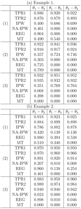
Tables 2.2 (a) and (b) report the coverage probabilities of the 95% confidence
inter-val (C.I.) for the average treatment effects. For each MC sample and each (N, n), we
computed the point estimator bθ and the variance estimator of θb, and constructed the
95% C.I. for the pair differences. Variance estimation for the DE is similar to (2.47) with Vb2g replaced by N−2 P i∈A2g P j∈A2g(π1ijπˆ2ij) −1∆
1ij(π−1i1yig)(π1j−1yjg). Variance esti-mation for the NA-IPW was done by noting the NA-IPW estimator as a special case of the IPW estimator with assumed simple random sampling in the first phase. The
estimated variance of the REG and the MT are provided by the regression and matching packages used in R. Note that the variance estimators for the estimators ignoring the first phase probabilities are not appropriate and can be biased under the full design. In both examples, estimators NA-IPW and REG have very poor coverage probabilities due to the large biases. Estimators IPW and MT that do not ignore the first phase sampling underestimate coverage probabilities in both example and 2. Our two estimators, TPR1 and TPR2, give satisfactory coverage probabilities in both examples even for a small sample size, relative to the nominal size 0.95.
2.3
Conclusion and Remarks
Much of the focus of observational study analysis has been on incorporating treat-ment selection into estimators to reduce bias due to self selection. Ignoring the first-phase sample design can have large implications for the interpretation of data. Accounting for the first-phase sample design reduces the bias and makes the target of estimation explicit. By incorporating auxiliary variables, the proposed two-phase semiparametric regression estimators are an improvement over the IPW estimators in finite sample problems. The assumptions for the two-phase regression estimators are reasonable for a large number of problems and we demonstrate that valid inference can be made with semiparamet-ric model specificiations. However, these estimators only account for bias that can be explained by observed covariates. If the second-phase inclusion probabilities depend on unobserved variables, residual bias will exist. Further, the IPW and two-phase semi-parametric regression estimators rely on a known first-phase design. In some cases, the first-order inclusion probabilities may need to be estimated and a design such as Poisson sampling is assumed. In summary, consideration of handling sample selection phases prior to treatment selection and auxiliary variables can lead to stronger and clearer evidence from observational studies. Estimating treatment effect parameters defined
through a general estimation equation in observational studies is the topic in the next chapter.
Table 2.1 The MC biases, variances and MSEs of the estimated treatment ef-fects, for (1): (N, n) = (12500,250); (2): (N, n) = (25000,500); (3): (N, n) = (50000,1000).
(a) Example 1.
θ1−θ2 θ1−θ3 θ2−θ3
Bias Var MSE Bias Var MSE Bias Var MSE
TPR1 -0.008 0.309 0.309 -0.090 1.543 1.551 -0.082 1.495 1.502 TPR2 -0.008 0.353 0.353 -0.093 0.604 0.613 -0.085 0.562 0.569 (1) IPW 0.395 4.900 5.056 0.681 5.321 5.785 0.286 4.766 4.848 NA-IPW 2.138 2.312 6.883 12.259 3.104 153.395 10.122 2.554 104.999 REG 1.579 1.424 3.917 10.930 2.814 122.276 9.351 2.905 90.342 MT -0.731 6.032 6.571 -0.394 4.051 4.209 0.340 3.528 3.652 TPR1 0.002 0.129 0.129 -0.036 0.673 0.674 -0.038 0.690 0.692 TPR2 0.002 0.133 0.133 -0.023 0.241 0.241 -0.025 0.235 0.236 (2) IPW 0.109 2.298 2.310 0.169 2.136 2.165 0.060 1.882 1.886 NA-IPW 2.015 0.811 4.871 12.033 1.056 145.847 10.018 0.927 101.285 REG 1.616 0.623 3.236 10.954 1.238 121.229 9.338 1.250 88.439 MT -0.891 3.072 3.858 -0.543 2.041 2.342 0.348 1.773 1.891 TPR1 -0.001 0.064 0.064 -0.006 0.337 0.337 -0.004 0.332 0.332 TPR2 0.000 0.064 0.064 -0.012 0.117 0.117 -0.012 0.115 0.115 (3) IPW 0.040 1.080 1.082 0.070 0.911 0.916 0.030 0.874 0.875 NA-IPW 1.999 0.350 4.348 12.005 0.445 144.572 10.006 0.392 100.51 REG 1.613 0.292 2.895 10.903 0.590 119.465 9.290 0.608 86.904 MT -0.907 1.501 2.321 -0.581 0.972 1.311 0.330 0.861 0.971 (b) Example 2. θ1−θ2 θ1−θ3 θ2−θ3
Bias Var MSE Bias Var MSE Bias Var MSE
TPR1 0.081 1.349 1.356 0.193 6.629 6.667 0.112 4.539 4.551 TPR2 0.083 1.349 1.356 0.182 1.570 1.603 0.099 1.438 1.447 (1) IPW 0.138 1.504 1.523 0.814 7.425 8.087 0.676 4.855 5.312 NA-IPW 1.386 1.153 3.073 6.861 6.150 53.227 5.476 4.027 34.009 REG 1.086 2.742 3.922 5.546 8.208 38.971 4.460 6.777 26.668 MT -0.310 5.331 5.423 -0.534 8.031 8.324 -0.222 5.342 5.389 TPR1 0.008 0.273 0.273 0.087 2.817 2.824 0.079 1.815 1.821 TPR2 -0.011 0.185 0.185 -0.013 0.326 0.326 -0.002 0.232 0.232 (2) IPW 0.024 0.492 0.493 0.489 3.081 3.32 0.465 2.059 2.276 NA-IPW 1.344 0.378 2.183 6.838 2.583 49.337 5.494 1.717 31.902 REG 1.068 1.319 2.460 5.429 4.046 33.520 4.361 3.226 22.242 MT -0.35 2.668 2.789 -0.628 3.878 4.281 -0.276 2.800 2.881 TPR1 0.000 0.112 0.112 -0.030 1.319 1.320 -0.030 0.834 0.835 TPR2 -0.001 0.061 0.061 -0.023 0.120 0.121 -0.022 0.084 0.084 (3) IPW 0.039 0.165 0.167 0.206 1.429 1.471 0.166 0.918 0.946 NA-IPW 1.373 0.139 2.025 6.687 1.236 45.949 5.313 0.782 29.015 REG 1.149 0.621 1.941 5.410 1.954 31.223 4.261 1.603 19.761 MT -0.317 1.321 1.423 -0.581 2.021 2.349 -0.255 1.321 1.389
Figure 2.1 The plots of Monte Carlo averages (panel (a)) and root mean square errors (panel (b)) of estimated treatment means versus treatment levels in Example 1. (a) Mo nt e C arl o Ave ra ge o f t he Est ima te d Ma rg in al Me an s θ1=−2 θ2=0 θ3=2 -8 .0 -6 .0 -4 .0 -2 .0 0.0 1.5 3.0 4.5 (b) R oo t Me an Sq ua re Erro r of th e Est ima te d Ma rg in al Me an s θ1=−2 θ2=0 θ3=2 0.0 1.5 3.0 4.5 6.0 7.5 TPR1 TPR2 DE IPW NA True
Table 2.2 The coverage probabilities of the 95% C.I. for estimated treatment ef-fects, for (1): (N, n) = (12500,250); (2): (N, n) = (25000,500); (3): (N, n) = (50000,1000). (a) Example 1. θ1−θ2 θ1−θ3 θ2−θ3 TPR1 0.886 0.920 0.922 TPR2 0.876 0.879 0.893 (1) IPW 0.400 0.686 0.699 NA-IPW 0.461 0.000 0.000 REG 0.904 0.000 0.000 MT 0.490 0.540 0.000 TPR1 0.922 0.941 0.936 TPR2 0.916 0.917 0.924 (2) IPW 0.357 0.724 0.746 NA-IPW 0.303 0.000 0.000 REG 0.725 0.000 0.000 MT 0.789 0.000 0.000 TPR1 0.932 0.951 0.952 TPR2 0.935 0.932 0.932 (3) IPW 0.351 0.769 0.764 NA-IPW 0.068 0.000 0.000 REG 0.398 0.000 0.000 MT 0.000 0.000 0.000 (b) Example 2. θ1−θ2 θ1−θ3 θ2−θ3 TPR1 0.918 0.923 0.925 TPR2 0.884 0.899 0.898 (1) IPW 0.786 0.882 0.878 NA-IPW 0.420 0.139 0.136 REG 0.980 0.394 0.538 MT 0.510 0.340 0.000 TPR1 0.970 0.950 0.950 TPR2 0.970 0.960 0.966 (2) IPW 0.891 0.920 0.914 NA-IPW 0.207 0.010 0.008 REG 0.960 0.138 0.254 MT 0.461 0.000 0.000 TPR1 0.983 0.958 0.960 TPR2 0.989 0.974 0.984 (3) IPW 0.940 0.940 0.942 NA-IPW 0.023 0.000 0.000 REG 0.898 0.010 0.046 MT 0.000 0.000 0.000
Figure 2.2 The plots of Monte Carlo averages (panel (a)) and root mean square errors (panel (b)) of estimated treatment means versus treatment levels in Example 2. (a) Mo nt e C arl o Ave ra ge o f t he Est ima te d Ma rg in al Me an s θ1=5 θ2=5 θ3=5 1.0 2.0 3.0 4.0 5.0 6.0 7.0 8.0 9.0 (b) R oo t Me an Sq ua re Erro r of th e Est ima te d Ma rg in al Me an s θ1=5 θ2=5 θ3=5 0.0 1.0 2.0 3.0 4.0 5.0 6.0 TPR1 TPR2 DE IPW NA True
CHAPTER 3.
ESTIMATING MULTIPLE TREATMENT
EFFECTS USING GENERALIZED ESTIMATING
EQUATIONS
In this chapter, we propose a generalized method of moments (GMM) based estimator and an empirical likelihood (EL) based estimator using generalized estimating equations. The estimators estimate parameters of interest defined through generalized estimating equations, including these from marginal, proportional, and regression coefficient models. We use them to make causal inference on observational data with complex sampling designs. Propensity score methods that incorporate the first phase design and the second phase selection probabilities estimated by a semiparametric sieve algorithm are used in the GMM and EL approaches. In addition to the estimating equations adjusted by the propensity scores, we also add covariate information into the equation system to gain efficiency. We show that proposed estimators have smaller bias compared to the estimators that ignore the first phase design, and in general have slightly smaller variance than the inverse propensity weighted and the double expansion estimators. Simulation studies are provided to support our conclusion.
3.1
Introduction
Observational data are used extensively in both research studies and industrial prac-tice. Although experimental studies are taken as the gold standard in many fields, we know they might be inappropriate or too costly in certain fields, including health care
(Black 1996). Observational studies have been shown to be useful in smoking and health studies (Rosenbaum 2002) when controlled experimental studies are not ethical. Besides, observational data have good features, like large sample sizes and timely access. It is not uncommon to see multiple treatments in observational data (Yu, Legg, and Liu 2013). Furthermore, the treatment selection is often a non-controlled selection process. These features result in a selection bias problem. Although matching methods (Rubin 1973) and propensity score methods (Rosenbaum and Rubin 1983) can eliminate the selection bias in making causal inferences, they mainly deal with only two treatments. Also, the data might be a survey sample coming from a population with unequal weights, and ignoring the survey design results in biased estimations (Yu, Legg, and Liu 2013). We need an estimator to handle survey sample data with multiple treatments. Chapter 2 has proposed a two-phase regression estimator to unbiasedly estimate marginal treat-ment effects in a multiple treattreat-ment situation. In Chapter 3, we propose estimators to estimate treatment effects in a more general set up, which are defined through estimat-ing equations. We will introduce two methods: one is based on generalized estimatestimat-ing equations and the other one is based on empirical likelihood.
Generalized method of moments has been used extensively since its invention for estimating parameters defined through a General Estimating Equation (GEE). Hansen (1982) provided the large sample theory of consistency and normality for these estima-tors. Pakes and Pollard (1989) derive efficient estimators and present detailed proofs of consistency and normality properties. The empirical likelihood method proposed by Owen (1988) is also widely used for solving a GEE. Qin and Lawless (1994) include the generalized estimating equations in an empirical likelihood method. It is common that data sets available in reality are from a survey design with unequal weights. Also, using such observational data sets to make statistical causal inference may be invalid due to selection bias. Here we assume the ignorable missing mechanism, which is commonly adopted by many researchers. With this assumption, the selection bias is removed by
the propensity score method (Rosenbaum and Rubin 1983). Hirano, Imbens and Ridder (2003), and Cattaneo (2010) extended the propensity score to the generalized propen-sity score in order to handle multiple treatments estimation. The inverse probability weighted (IPW) estimation proposed by Hirano, Imbens and Ridder (2003) is consid-ered here. The double expansion (DE) estimator, an improved estimator that considers the first phase design, is also included in this discussion. Sieve approximation is used to approximate propensity scores without known functional forms. However, as yet we have not found one method that can deal with unequal weights in data, which is crucial in removing estimation bias when informative sampling exists. Also none of them uses extra moments created by covariates to reduce the variation of estimators.
In both GMM and EL frameworks, the estimating equations are adjusted by propen-sity scores that consider both the first phase sampling probabilities and the second phase selection probabilities as estimated by Cattaneo (2010). We add additional covariate mo-ments and group moment functions to gain efficiency. We show that without considering first phase weights when they are present the estimation biases may be large. The proof of consistency and normality of the extended estimator are provided. Estimators, including Cattaneo (2010)’s Inverse Propensity Weighted and Double Expansion estimators, are compared to the proposed estimator. Closed form variance estimators are also provided to make statistical inference.
We organize this chapter as the follows. Section 3.2 proposes the GMM estimator, and Section 3.3 proposes the EL estimator. Simulation studies are provided in Section 3.4. Conclusions are presented in Section 3.5.
3.2
Basic Set Up and the Proposed GMM Estimator
3.2.1 The Proposed GMM Estimator
We set U as a realized finite i.i.d. population from an infinite superpopulation S.
U contains information on (Yi, Xi), where i = 1, ..., N indexes each individual, and
Yi = [yi1, ..., yiG]T whereG is the number of available treatments for each unit. A vector of covariates Xi is used in regression and calibration, and Yi is related to Xi by a model
function. We assume we only observe a first phase sample A1 from the population U.
The observed sample has a sample size n and informative unequal survey weights. We
use δ1i and δ1ij to denote selection indicators in the first phase design:
δ1i =
1 if uniti is selected in the first phase A1; 0 otherwise. (3.1) δ1ij =
1 if unit i and j are selected in sample A1 simultaneously; 0 otherwise.
(3.2)
In each unit from the first-phase sample, Xi is observed fully; however, one and only one Yig is observed due to individual treatment selection. We use the indicator variable
δ2ig to indicate unit treatment selection conditional on its selection in the first phase A1,
δ2ig =
1 if unit i selected treatment g; 0 otherwise. (3.3) Consequently, we have G P g=1
δ2ig = 1 for i= 1, ..., n. This indicator variable partitions the first phase sampleA1 to disjoint second phase samplesA21, ..., A2G, with δ2ig = 1, for all units in A1, g = 1, ..., G. We assume we know the first phase selection probabilities
π1i and joint selection probabilities π1ij, and we have E(δ1i|U) = π1i and E(δ1ij|U) =
Then, the treatment selection δ2ig is conditionally independent with Yi when observing covariates Xi in sample A1. Thus we have the relationship
δ2ig ⊥Yi |Xi (3.4)
To make valid causal inferences using observational data, we plan to use the propen-sity score (Rosenbaum and Rubin 1983) to adjust the selection bias. In the second phase sample, the conditional treatment selection probabilities π2ig =E(δ2ig|X) are unknown. They can be taken as a generalized propensity score introduced in Hirano and Imbens (2004). We adopt the algorithm used in Cattaneo (2010) to estimate multiple propensity scores π2ig. Under suitable regularity conditions, we have the estimated ˆπ2ig (Yu, Legg and Liu 2013) as below,
ˆ π2ig = exp(RTK(Xi)ˆγg) G P h=1 exp(RT K(Xi)ˆγh) (3.5)
whereRK(Xi) is a spline approximation function usingXi, and ˆγ= (ˆγT1, ...,γˆ T G)T is from ˆ γ = arg max γ|γ1=0 X i∈A1 G X g=1 δ2iglog exp(RT K(Xi)γg) G P h=1 exp(RT K(Xi)γh) , (3.6)
Under the same regularity conditions, ˆπ2ig converges toπ2ig in certain speed (Yu, Legg and Liu 2013). There is no functional assumption for the propensity scores π2ig, except its relation to Xi; we thus call this estimating algorithm a semiparametric method.
In the regular generalized method of moments estimators, all variables involved in the estimating equations are assumed to be observed in sample. Here we assume we observe
X in a sampleA1, butYiis only observed in the selected treatment for each uniti. Thus, we need to incorporate survey weights of the first phase and the selection probabilities of the second phase into the propensity scores that are applied to the estimating equations
to correct the sampling and selection bias. Additional informationXi is incorporated to gain potential efficiency.
Define ¯X1π = N1 P i∈U Xiδ1i π1i , ˜X2πg = 1 N P i∈U Xiδ1iδ2ig π1iˆπ2ig , ˜m2πg(θ) = 1 N P i∈U mig(θ)δ1iδ2ig π1iˆπ2ig , and G(θ) = E(X)−µ E(X)−µ .. . E(X)−µ E(m1(β)) .. . E(mG(β)) (3.7)
The reason why we have multipleE(X)−µis that we consider using theX covariates in both the first-phase sample and the second-phase sample. Thus the asymptotic expecta-tions of the estimating equaexpecta-tions from different treatments are the same asE(X)−µ. We can see this through the following estimating equations. Here an interested parameter
θ0 is defined as the unique solution of G(θ) = 0. Set
GN(θ) = ¯ X1π −µ ˜ X2π1−µ .. . ˜ X2πG−µ ˜ m2π1(β) .. . ˜ m2πG(β) (3.8)
Then the proposed estimator is
ˆ
θN = arg min θ