Annales UMCS Informatica AI 7 (2007) 61-71
Annales UMCS
Informatica
Lublin-Polonia Sectio AI http://www.annales.umcs.lublin.pl/Global models of dynamic complex systems – modelling using
the multilayer neural networks
Grzegorz Dra
á
us
*Faculty of Electrical and Computer Engineering, Rzeszów University of Technology, W. Pola 2, 35-959 Rzeszów, Poland
Abstract
In this paper, global models of dynamic complex systems using the neural networks is discussed. The description of a complex system is given by a description of each system element and structure. As a model the multilayer neural networks with the tapped delay line (TDL), which have the same structure as a complex system, are accepted. Two approaches, a global model and a global model with the quality local model taken into account are proposed.
To learn global models the modified back-propagation algorithms have been developed for the unique structure of the complex model. To model dynamic simple plants, of which the complex system is composed, a series-parallel model of identification using the feedforward network with the tapped delay line (TDL) and the feedback loops, in which the gradient can be calculated by means of the simpler static back-propagation method is proposed. Computer simulations were performed for the dynamic complex system, which consists of two dynamic nonlinear simple plants connected in series, described by means of nonlinear difference equations.
1. Introduction
There are various of kinds of complex systems. The first kind is composed of blocks (simple plants), consisting of identification of particular process blocks and their interconnections [1]. The other one is a collection of systems that are not approximable (arbitrarily close) by a finitely parameterized collection of systems [2]. Another example are the complex systems as the complex operation ones [3].
In this paper the dynamic complex system, is a system which consists of dynamic simple plants connected in the internal structure of the system, that means the flow of signals between particular simple plants. Simple plant means the input-output system.
*E-mail address: [email protected]
Modelling methods of dynamic systems are well known and extensively represented in literature. However, modelling of dynamic complex systems is a very difficult problem and not solved so far. For example, in the complex control of industry processes it is necessary to specify the control algorithm for different phases of the process. Developing models of complex systems is forced by the need for complex control of complex industrial systems [1].
Mathematical methods of the complex system identification are usually based on the modelling of simple plants being parts of complex systems and on their optimisation. Then, the model of a complex system consisting of optimal simple models is built up. However, such models are not global models [1].
The main goal of this paper is to show that it is possible to achieve global models of dynamic complex systems using the multilayer neural networks with the feedback loop.
One of typical complex systems is the collection series connecting simple plants without the feedback loop. In this structure the output preview of a simple plant is the input to the next simple plant. So, the global model of the complex system is obtained by connecting simple models in the same series (cascade) structure. Output signals of simple models and simple plants, and output signals of the global model and the complex system will be used to construct a quality criterion of the global model. Two cases will be taken into account, depending on the way of considering a particular simple model in the global model. The first case is the global model, in which signals flow during the learning mode and working modes are the same as in the complex system. The global model has the same structure as the complex system. For this model the global quality criterion was defined. Adjusting parameters for this model (learning of the net) should be done in such a way that the model outputs are close to the complex system outputs, in the same structure. The second task is the difference between the simple model outputs and the simple plant outputs should be small.
The second case is the global model with the quality of local models taken into account. The quality of local models in a global model can be considered by the acceptance of the synthetic criterion. This criterion assures that the global model will be satisfactory and local models which the global model consists of, will have sufficiently good quality. Both models have the same structure but they differ in the way of learning.
2. Models of complex systems
For the modeling of simple dynamic plants with multilayer neural networks, usually the series-parallel model is used [6]. In a such structure, present and past input and output signals transmitted via TDL are used. In this case there is no feedback from the network, but from the plant. Then, the neural network works
as an unidirectional one and it can be learned according to the “delta” rule (the static backpropagation algorithm). After the learning phase (stage), if the error of modeling is sufficiently small, the series-parallel model can be replaced by a parallel model with the feedback loop from the model outputs without significant consequences [6].
2.1. The global model of the dynamic complex system (GM)
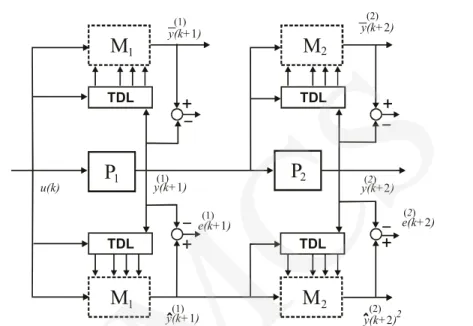
The dynamic complex system can consist of R simple plants. An example of a complex system which consists of two simple plants (R = 2) and its global model is shown in Fig. 1. The global model which consists of two simple models (noted as M1 i M2), is connected in the structure corresponding to this system. In
such a structure the output preview simple model is the input to the next simple model. The outputs of a global model are described:
( ) ( 1) ( ) (1) (1) ( 1) ( ) 1 1 (1) (1) ( ) ˆ ˆ , , , , , ˆ , , , r r r r r r r r r r f f f f f y y w u w w w u w w " " ! , (1)where: u(1) is the external input for the global model and the complex system, w(r) are the parameters (weights) of r-th simple model.
Passing on the input of the model k-th sample of input vector u(1)(k) we get the output signals of the r-th simple model ( ) ( ) ( )
1 2 ˆ r ( ) [k yˆ r ( ), ( ), k yˆ r k , y " ( ) ˆ ( )] r r J
y k , where Jr is the number of outputs of the r-th simple model.
The error for k-th learning data sample for the r-th simple model is as follows:
ˆ r k ˆ r k r r k r
e y y . (2)
The global quality assessment criterion for this global model is the sum of squared errors (differences) between the outputs of simple models (Mr) and the
outputs of respective simple plants (Pr) of the complex system:
T 1 1 1 ˆ ˆ 2 R K r r g r g r k Q W¦
EQ w¦
e k ȕe k , (3)and the quality assessment criterion of a simple model in the global model:
2 1 1 1 ˆ 2 r J K r r r r g j j k j Q w¦¦
y k r y k r , (4)where: E = diag[E1,E2,…,ER], Er [0,1], r = 1,…,R and
¦
Rr 1Er 1, K – thelength of input vector, W = {w(1),w(2),…,w(R)} – is a set of parameters (weights)
of the global model divided into subsets of simple models.
u(k)
P
1 y(k+ )1P
2 2M
TDL y(k+ )2 ( )2 (2) (1) ( )2 e(k+ )2+
y(k+ )2 y(k+ )1+
TDL e(k+ )1 (1) (1)+
1M
M
2 1M
TDL TDL (2) y(k+ )22 y(k+ )(1)1+
Fig. 1. The two-parts complex system and their global models
The coefficients ȕr determine the effect of individual simple models on the
global quality criterion.
As a global model the multilayer neural networks with TDL were accepted. To determine these optimal model parameters W the modified backpropagation learning algorithm for the dynamic complex systems presented in detail in [5] can be used.
2.2.The global model for dynamic complex system with the quality local models taken into account
In the global model with the quality local models taken into account the compromise between the global model quality and local models quality is to be found. Parameters of such a model should ensure that the global model is satisfactory and local models are of sufficiently good quality.
For the complex system shown in Fig. 1 there is built the global model which has the same structure. In the global model there can be pointed out the local models, which are denoted as M1 and M2. The outputs y( )r of the local models
are described by the formula:
,r r r
r
f
y u w , (5)
where the input of the r-th local model u(r) = y(r–1) is the output of the previous
simple plant.
The error of the r-th local model for the k-th learning data sample is as follows:
r k r r k r r k r
e y y . (6)
The differences between the outputs of local models (Mr) and those of
respective simple plants (Pr) of the complex system are used to define the quality
criterion of local models :
T 2 1 1 1 1 1 2 2 r J K K r r r r r r j j k k j Q w¦
e k e k¦¦
y k r y k r . (7) For the global model with respect to the quality of local models, the synthetic criterion was accepted:1 0 1 1 r R w g r r R R Q W D Q W D Q w " D Q w "D Q w , (8) where: 0 dDrd 1 for r = 0,1,…,R, 0 1 R r r D
¦
.The coefficients D = [D1D2 … DR] determine the effect of individual local
models on the synthetic quality criterion (8). The coefficient D0 determines the
effect of global quality criterion (3) on the synthetic quality criterion (8). By suitable choice of Dr coefficients the influence of the local models on the global
model can be determined.
2.3. Modified backpropagation learning algorithm for the global model with quality local models taken into account (GLM)
For learning the multilayer neural networks, of which the GLM model is constructed, it was necessary to modify the well-known gradient error backpropagation algorithm. This modification must consider the situation that a complex model consists of the static network with the tapped delay line and the feedback loop form a complex system during the learning mode and the feedback loop forms the complex model when the model works.
The synthetic quality criterion (8) for the k-th data learning sample can be written as:
2 , 0 1 2 1 1 1 ˆ 2 1 . 2 r r J R R k k w R j j j J R r r r j j r j Q y k R y k R y k r y k r D E D¦
¦ ¦
W (9)In criterion (9) (model GLM) all coefficients Er are equal zero, except for the
last one ER = 1. In order to minimise the error function Qwk( )W , the gradient
descend method can be now applied. Using this method for the neural network learning, one obtains the following weight increment:
m k k j w w ji m ji j ji z Q Q w k w z w w w w K K w w w ' W W , (10)
when: K – the learning rate from the range (0.1).
Let us define the „delta” error įj(r),m,k arising in j-th element of m-th layer in r-th element of the model for k-th sample:
, , m k k k j r m k w w w m j m m m m j j j j j u Q Q Q f z k z k u k z k u k w w w w G w w w w c W W W , (11) where ( )m ju k is the output signal of j-th neuron of m-th layer of network, m( )
j
u k
= ˆm( )
j
u k in the global model and m( )
j
u k = m( )
j
u k in local models.
At this point, one has to introduce the concept of the “additional” hidden layers. The “additional” layers are those whose outputs are also the outputs of sub-models.
Omitting the calculation details, the „delta” errors for particular layers can be calculated as follows:
– for the output layer,
, , 0 ˆ R M k M R R j j j j R R M R j j j f z k y k R y k R f z k y k R y k R G D D c c (12)– for the common hidden layer:
1 , , , , 1, , 1 1 m I r m k m k r m k r m j j l lj l f z w G c
¦
G , (13)– for the “additional” hidden layer:
1 , , 1 , 1 , 1 , 1 1 , m I r m k m r m k r m j j l lj l r r m k r j j j f z k w f z y k r y k r G G D c c¦
, (14)With the above definitions, the general delta formula for weight increments takes the form:
, , , 1 , , 1 1 1 ˆ K K r m r m k m r m k m ji j i j i k k w K G u k r K G u k r '¦
¦
. (15)The Rprop algorithm [7], which does not use the information about the values of gradients allows for the significant increase in the speed of the learning process, especially in the areas where the error function gradient is not steep. The adjustment of the parameters in the l-th step of optimization in the modified
Rprop method is:
¦
¦
¦
(16) where 1 1 max 1 1 min 1 1 min , for 0 max , for 0 for 0 l l l l ji ji ji l l l l l ji ji ji ji l l l ji ji ji a S S b S S S S K K K K K K ! ° ° ® ° ° ¯ (17) (17) and l – the number epoch, l ( ( ))ji w ji
S wQ Wl ww ; a=1.2; b=0.5; Kmax = 50;
Kmin = 10-6 are taken from [8].
3.Simulations
For modelling, a dynamic nonlinear complex system has been selected, consisting of the serial connection of two dynamic nonlinear simple plants described by the second-order nonlinear difference equations:
1 1 1 2 1 1 , 1 , ( 2), , ( 1) y k f y k y k y k u k u k , (18) 2 2 2 2 1 1 2 2 1 , , 1 , 1 , y k f y k y k y k y k y k , (19)where the nonlinear functions f1 and f2 are given by the formulae:
1 2 3 5 3 4 1 1 2 3 4 5 2 2 2 3 1 , , , , 1 x x x x x x f x x x x x x x , (20) 2 3 5 1 4 2 1 2 3 4 5 2 1 1 , , , , 1 2 v v v v v f v v v v v v . (21)The system input and the model input of the learning signal is given by:
sin 2 / 50 for 0 250
u k Sk d dk .
The system input and the model input of the testing signal is given by:
sin 2 / 250 for 250
0.8sin 2 / 250 0.2sin 2 / 25 for 250 500
u k k k u k k k k S S S d d
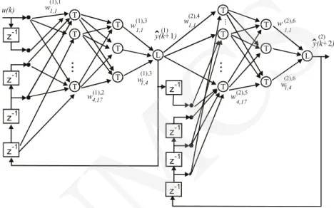
As the global model (GM) and the global model with the quality of local models taken into account (GLM), the 6-layer feedforward neural network (see Fig. 2) of the following structure has been adopted: 5 network inputs; 17 neurons (of the hyperbolic tangent transfer function) in the first hidden layer; 4 neurons
in the second hidden layer; 1 linear neuron in the “additional” (third) layer; 17 and 4 neurons in the fourth and the fifth layers, respectively; 1 linear neuron in the sixth (output) layer of the complex model (shortly, 1(5)-17-4-1(4)-17-4-1).
u(k) T y(k+ )2 w w w w w w w w (1),1 1,1 y(k+ )(1)1 (1),2 4,17 (1),3 1,4 (2),5 4,17 (2),6 1,4 (2),6 1,1 (2) (1),3 1,1 (2),4 1,1 T T z-1 T T T T T T T T T L L z-1 z-1 z-1 z-1 z-1 z-1 z-1
Fig. 2. The neural network as the (parallel model – working mode) global model (GM) of the complex system
The following values of the factors of formula (3) in the GM model have been arbitrarily adopted: ȕ1 = 0.5, ȕ2 = 0.5. The following values of the factors of
formula (7) in the GLM model have been arbitrarily adopted: E1 = 0, E2 = 1,
D0 = 0.5, D1 = 0.25, D2 = 0.25.
For learning all the models the modified gradient with the learning rate
K= 0.001 and the modified Rprop algorithm were used. The adjustment of parameters was performed by computing gradient of the averaged error function for all 500 discrete time samples.
As an additional criterion of modelling quality assessment, the relative percentage error RPE (22) has been adopted and calculated for each output of
r-th model: 1 1 ˆ RPE 100% K r r k r K r k y k y k y k
¦
¦
. (22)Results of modeling in the form of values of the global criterion Qg, synthetic criterion Qw, the local criteria Q2, Q1 and the simple model criterion Qg(2) (where
(1) 1
g
Q Q ) after 500 epochs of learning, are shown in Table 1 for both
series-UMCS
parallel (feedback from the plant) and parallel (feedback from the model) models. The values of RPE after 500 learning epochs are presented in Table 2.
Table 1. Quality criteria after 500 learning epochs
Criterions Qg/Qw Q1 Q2 Qg(2) Qg/Qw Q1 Q2 Q(2)g
Models Learning – series-parallel model Testing – parallel model
GM – gadient alg. 0.509 0.503 - 0.516 0.352 0.243 - 0.470 GLM – gradient alg. 0.428 0.387 0.561 0.382 0.449 0.405 0.519 0.4360 GLM – Rprop alg. 0.0147 0.0352 0.0127 0.0054 0.0614 0.144 0.0143 0.0435 GM – Rprop alg. 0.0294 0.0366 - 0.0222 0.1710 0.273 - 0.0679 GLM – grad. (2000 epoch) 0.117 0.172 0.124 0.086 0.312 0.404 0.246 0.299
Table 2. RPE after 500 learning epochs for testing data for parallel model Number of output r = 1 (locally)r = 2 r = 2 R = 1 (locally) r = 2 r = 2
for gradient algorithm for Rprop algorithm
Models [%] [%] [%] [%] [%] [%]
GLM 4.83 8.92 7.42 2.79 1.36 2.19
GM 3.55 - 8.16 3.77 - 2.78
The errors in the parallel model for the same epoch number are much smaller by using the Rprop algorithm than using the gradient algorithm for the learning.
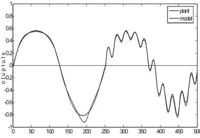
0 50 100 150 200 250 300 350 400 450 500 -1 -0.8 -0.6 -0.4 -0.2 0 0.2 0.4 0.6 0.8 1 o t u p t u t s plant model
Fig. 3. The outputs of the first local model of GLM and the first simple plant for the testing data
The errors of external outputs of the GM model are bigger than those in the GLM model for both kinds of algorithm. In the GLM model the errors of the output of the second local model (r = 2) are lower than those of external output of that model for the Rprop algorithm (for gradient after 2000 epoch learning).
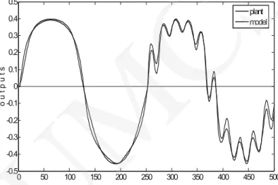
Testing signals in the GLM model for gradient algorithm after 500 epoch of learning are shown in Figs. 3 and 4.
0 50 100 150 200 250 300 350 400 450 500 -0.5 -0.4 -0.3 -0.2 -0.1 0 0.1 0.2 0.3 0.4 0.5 o u t p u t s plant model
Fig. 4. The external outputs of the GLM model (parallel model) and the complex system for the testing data
Conclusions
In the paper the results of computer simulation for the global model (GM) and the global models with the quality of local models taken into account (GLM) are presented. The quality (accuracy) of the GM model and the GLM model are satisfactorily good. The modified Rprop algorithm was much faster than the modified gradient backpropagation algorithm which needed the acceptance of a very small learning rate due to many learning samples. Learning for both discussed algorithm was in reasonable time.
The presented results confirm the possibility of developing global models of dynamic complex systems using the static multilayer feedforward neural networks with TDL.
Further work is to use the proposed method of the neural networks which are the universal approximators and the modified learning algorithms to model a complex system with difficult or unknown dynamic. It is for modelling a number of plants, which can have many inputs and many outputs.
References
[1] Bubnicki Z., Identification of Control Plants, Oxford, Amsterdam, N.York: Elsevier, (1980). [2] Dahleh M.A., Venkatesh Sr., System Identification for Complex Systems: Problem
Formulation and Results, In Proceedings of the 36th IEEE Conf. on Dec. and Control, (1997). [3] Józefczyk J., Decision making problems in complex of operations systems, Wrocáaw
University of Technology Press, Wroclaw, (2002), in Polish.
[ 4 ] Draáus G., ĝwiątek J., Globally optimal models of complex systems with regard to quality local models. Proceedings of 14th “International Conference on Systems Science”, Wrocáaw,
(2001), 217.
[5] Draáus G., Modeling of Dynamic Nonlinear Complex Systems Using Neural Networks.
Proceedings of the 15th “International Conference on Systems Science”, Wrocáaw, III, (2004),
87.
[6] Narendra K.S., Parthasarathy K., Identification and Control of Dynamic Systems Using Neural Network, IEEE Trans. On Neural Networks, 1(1) (1990) 4.
[7] Riedmiller M., Braun H., RPROP – a fast adaptive learning algorithm, Technical Report, University Karlsruhe, (1992).
[8] Zell A., SNNS – Stuttgart Neural Network Simulator, User Manual, Stuttgart, (1993).