Applying Multiple Particle Swarm Optimization Algorithm to the Optimal Setting of Time Coordination Curve of FTU in Distribution Feeder Automated System

(1)



Abstract— In this study, mathematical optimization was

applied to improve the fault interval assessment of feeder terminal units (FTUs). Because of the insufficient hardware computing power in such units, using a time coordination curve to calculate fault curves leads to the occurrence of jagged curves. Such jagged curves lead to considerably high errors, ultimately resulting in malfunction or erroneous nonoperation. A multi-particle swarm optimization (multi-PSO) algorithm was proposed for resolving the malfunction caused by protection curves with considerably high errors. This algorithm improves the early convergence problem encountered in the original standard PSO algorithm and the long calculation time observed in the area method. When the proposed multi-PSO algorithm is applied in the optimization process, the arrangement of the nodes on the jagged curves improved; this results in the jagged curves exhibiting relatively smooth and curved outlines, thereby eliminating malfunctions and achieving upstream and downstream protection coordination as well as completing fault interval identification procedures. The main contribution of this study is the improvement of the erroneous assessment of distribution line faults observed in FTU fault flags. The proposed method also improves the success rate of FDIR in feeder automation systems.

Index Term— Fault diagnosis isolation restoration (FDIR),

Feeder automation, Feeder terminal unit (FTU), Multi-particle swarm algorithm, Protection coordination.

I. INTRODUCTION

TO improve the power supply quality and shorten the outage time, the Taiwan Power Company (Taipower) has established feeder automation systems on its distribution network. During persistent faults in the distribution system, the expert system for fault diagnosis isolation restoration (FDIR) within the feeder automation systems determines the fault site and isolates the interval of the incident according to the fault flag generated by the feeder terminal unit (FTU). The load of the distribution system is then analyzed so that it can be used to restore power upstream and transfer power downstream while maintaining adequate supply quality. This shortens the outage interval and reduces user outage time, improving the operational efficiency of feeder automation systems [1].

FTU fault flagging involves using a time coordination curve (TCC) for detecting and assessing faults. A key influence on

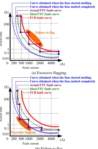
whether an FTU can flag faults appropriately is its method of calculating the TCC. Because FTU hardware has insufficient computing capability, TCC fault curves are not exhibited as consecutive points arranged in an arc shape. Rather, nodes on a jagged curve are used to detect fault current. However, using jagged curves for detecting fault current often results in considerably large errors, preventing upstream-downstream protection coordination. Thus, when an FTU detects fault current, abnormalities such as excessive flagging or failure to flag occur as shown in Fig. 1. Failure to flag often leads to equipment meltdown, whereas excessive flagging usually causes power outages. Inadequate fault flagging accuracy also prevents the FDIR expert system in the feeder automation system from executing its proper function when feeder incidents occur. Thus, the system or the dispatcher misjudges the incident interval, which expands the incident range and severely affects the quality of the power supplied to users.

Numerous studies have applied particle swarm optimization (PSO) to seek optimal solutions; for example, PSO algorithms have been applied to power flow problems involving distributed generator failures, to the design of power system stabilizers, and to the determination of optimal positions for deploying voltage measurement equipment in power system planning [2]–[4]. However, few studies have applied PSO to solve TCC optimization during faults. Taipower currently uses a rule-of-thumb approach through human-machine interfaces to address the optimization of FTU fault curves. This approach usually results in malfunctions induced by excessive flagging or failure to flag [5]. In addition, most studies have solved and compared the optimization of correlation curves, such as linearly decreasing curves, exponential curves, parabolic curves opening upward, fuzzy curves, and random curves, by using various PSO algorithms [8], [9]. After feeder faults are diagnosed, the fault position must be confirmed and isolated. At this time, an accurate TCC must be set to isolate the fault segment appropriately. The curve type in this situation is primarily an inverse time-current coordination curve. Although PSO can be used to obtain the solution for this type of curve in a relatively quick manner, it results in premature convergence and local optimal solutions [9]. In the current study, a multi-PSO algorithm was applied to derive optimal solutions. In the proposed method, a secondary standard particle swarm

Applying Multiple Particle Swarm Optimization

Algorithm to the Optimal Setting of Time

Coordination Curve of FTU in Distribution

Feeder Automated System

(2)

algorithm is executed to derive global optimal solutions while investigating optimal TCC set points.

(S)

(A) 0 200 500 1000 2000 4000 0.01

0.1 1 10 100

Fault current

Failure to flag FCB fault curve

Curve obtained when the fuse melted completely

Ideal FTU fault curve

Actual FTU fault curve

Curve obtained when the fuse started melting

A

ct

io

n

t

im

e

(a) Excessive flagging.

(S)

(A) 0 200 500 1000 2000 4000 0.01

0.1 1 10 100

Fault current

A

ct

io

n

t

im

e

FCB fault curve

Excessive flagging

(b) Failure to flag.

Fig. 1. Excessive flagging and failure to flag for fault detection.

II. FDIREXPERTSYSTEMINTHEFEEDER

AUTOMATION OF DISTRIBUTIONSYSTEM

To alleviate outage incidents, Taipower has repaired feeders manually in recent years. During such repair processes, field personnel often experience accidents, repair times are excessively long, and users are inconvenienced. To ameliorate these problems, Taipower is currently introducing an FDIR expert system into its feeder automation promotion system, the Siemens SINAUT Spectrum 4.4. This system is projected to increase power quality [6], shorten the outage time, and reduce accidents experienced by field personnel.

The FDIR expert system uses supervisory control and data acquisition (SCADA) to optimize feeders to upgrade the database. Distribution feeders having environmental geographic maps as blue plates are added to the SCADA database within the feeder optimization system. This facilitates the process of monitoring actual distribution feeders because the maps of such distribution feeders are available within the system database. The FTU calculates nodes to determine the fault curve. When the curve of the fault current is consistent with the fault current curve determined by the FTU, the FTU returns a fault flag to the master station, as shown in Fig. 2-(a). An environmental geographic map among the SCADA functions is then used to judge the location of the incident, as shown in Fig. 2-(b). Next, an automatic command instructs the

FTU to execute the automatic line switch to isolate the incident segment, as shown in Fig. 2-(c). After the incident segment is isolated, the system automatically sends a control command to the remote terminal unit of the substation to input the feeder circuit breaker (FCB). This enables the sound segment upstream of the incident segment to restore power. Finally, the load of the distribution system downstream is analyzed by using a transfer feeder that in principle has the same alternating voltage and substation as that of the distribution system as well as having a sufficient load capacity. This enables the distribution system to recommend a transfer plan for the restoration of downstream power while maintaining adequate power quality. The dispatchers on duty at the Taipower feeder dispatch control center reference this plan, enabling power to be restored in sound downstream segments, as shown in Fig. 2-(d). This shortens the outage interval, reduces user outage time, and improves the operational efficiency of feeder automation.

FCB

Control centre

FTU FTU FTU

FTU

Incident

Fault flag Fault flag A Substation

B Substation

(a) Fault flag is generated (F).

FCB Trips

FCB

Control centre

FTU FTU FTU

FTU

Incident interval

Fault flag Fault flag A Substation

B Substation

(b) Fault is detected automatically (FD).

FCB Trips

FCB

Control centre

FTU FTU FTU

FTU Fault flag Fault flag

Incision Incision

A Substation

B Substation

Incident interval

(c) Fault is isolated automatically (I).

FCB Input

FCB

Control centre

FTU FTU FTU

FTU Fault flag Fault flag

Input

A Substation

B Substation

Incision Incision

Incident interval

(3)

III. PROBLEMFORMULATION

A. Planning of the FTU Fault Curve in the Feeder Automation

System

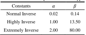
The FTU fault curve for the Taipower feeder automation system is currently formulated based on the fault curve equation of the intelligent electronic device (IED) embedded in the FCB of each substation. In (1), the fault curve of the REF-541 IED relay produced by ABB is used to formulate the FTU fault curve. According to Taipower’s secondary substation protection coordination provisions and British Standards 142 or International Electro technical Commission (IEC) 60255-4 standard, parameters associated with the extremely inverse curve type shown in Table 1 are used for formulating the FTU fault curve [10]–[12].

( )

()

(1)

In this formula,

( ): Action time (s).

: Adjustable time multiplier (this can generally be considered as the lever; that is, the set time value).

: Phase current (A) (this can be considered as the actual current or the test current).

: Adjustable current pick-up value (A) (this can generally be considered as the tap; that is, the set current value). and : constants. Their values indicate the curve type used

(Table I).

Table I

Parameters for the IED protection curve types.

Constants

Normal Inverse 0.02 0.14

Highly Inverse 1.00 13.50

Extremely Inverse 2.00 80.00

Most of the protection relays in FCBs have been modified from traditional mechanical protection relays to IEDs. The IED test manual indicates that the error value of the action time for the pick-up current value, , is within ±10% [7] and the error value of the hardware response time of the FTU fault curve is within ±10%. To prevent the error value of the coordination time from affecting the protection coordination between the FCB and FTU curves, the maximum error value of the protection time of the two curves must be 20% (Fig. 3). This value is used to set the FTU fault curve by using (2), achieving the provisions for upstream and downstream protection coordination. This error parameter can also be adjusted manually.

( )

()

(2)

(S)

(A) 0 200 500 1000 2000 4000 0.01

0.1 1 10 100

Fault current

FCB fault curve (backup protection)

Curve obtained when the fuse started melting (primary protection) Curve obtained when the fuse melted completely (primary protection)

FTU fault curve

Coordination time >20%

A

ct

io

n

t

im

e

Fig. 3. FTU fault curve planning positions.

B. FTU Fitness Function

The fitness function is used in optimization processes for determining the figure of merit. In this study, the jagged area between the ideal FTU fault curve and the actual FTU fault curve were used to determine the figure of merit. Fig. 4 shows that the FTU fault curve is enhanced as the jagged area diminished.

As shown in Fig. 4, points a, b, c, and d on the FTU fault curve are hardware nodes and correspond to the size of the fault current on the x-axis. To obtain the optimized FTU fault curve, fixed values must be set for points a and d on the curve. The fitness functions of points b and c are then obtained to determine the figure of merit.

(S)

(A) 0 200 500 1000 2000 4000 0.01

0.1 1 10 100

Fault current a

b

c

d

FCB fault curve

A

ct

io

n

t

im

e

Fig. 4. FTU Fitness Function.

To obtain the fitness function of point b in the ith particle swarm, points a and c must be set to fixed values. The integrals of the area under the curves formed by points a– b and points b– c are then calculated. The integral of the hatched area under the curve formed by points a–b is calculated using (3), whereas that of the curve formed by points b–c is calculated using (4). In these formulae, t = 1, 2, 3, …, m is the number of iterations, i = 1, 2, 3, … and n is the particle swarm [9].

∫ ( ) ( )

(3)

∫ ( ) ( )

(4)

The integral areas of (3) and (4) are then added as shown in (5). As the area of decreases, the fitness function of point b

in the ith particle swarm becomes enhanced.

(5)

To determine the fitness function of point c in the ith particle swarm, points b and d must first be set to fixed values. The integral of the shaded area under the curve formed by points b– c is calculated using (4), whereas that of the curve formed by points c–d is calculated using (6).

∫ ( ) ( )

(6)

The integral areas of (4) and (6) are then added as shown in (7). As the area of decreases, the fitness function of point b

in the ith particle swarm becomes enhanced.

(7)

In the overall fitness function of the FTU fault curve, the entire jagged area formed by the ideal FTU fault curve and actual FTU fault curve is used to determine the figure of merit of the hardware nodes, as shown in (8).

(8)

The problem in this study can be solved using the optimized mathematical model shown in (9).

( )

(9)

Subject to 1. ( ) ( )

2.

In this formula, Constraint 1 indicates that points b and c must be located within the interval of the fuse complete melting curve and the FCB fault curve. Constraint 2 states that the time interval between the FTU fault curve and FCB fault curve must be at least 20% of the pu time value.

IV. DEVELOPMENTOFMETHODOLOGY

A. Standard Particle Swarm Algorithm

Three factors generally influence the direction of a particle at the next point in time: particle direction at the next point in time = particle direction at time t + optimal direction determined by the particle + optimal direction determined by the swarm. In 1998, Shi and Eberhart proposed an inertia weight w in their implementation of the standard PSO algorithm shown in (10). Various weight calculations can be used to update the

convergence speed automatically. The weight is generally initialized at 0.9 and declines linearly to 0.4.

₍ ₎ ₍ ₎₍₁₀₎

where

: Inertia weight.

: Speed of particle i at time t.

: Position vector of particle i at time t.

: Optimal position determined by particle i so far.

: Optimal position determined by the particle swarm so far. : Learning factor, also called the acceleration factor

_

weight of individual experience, typically set to 2. : Learning factor, also called the acceleration factor

_

weight of swarm experience, typically set to 2. : Random value within [0, 1].

: Random value within [0, 1].

When the inertia weight, w, is relatively high, the PSO algorithm can search for a wide range of values. When the inertia weight is relatively low, the PSO algorithm can search for a narrow range of values. Therefore, if a linearly decreasing inertia weight is used during the iterative calculation, such as that shown in (11), the PSO algorithm can exhibit excellent global search capabilities from the beginning and can quickly locate a region that is near the global optimal solution. In the later stages, it can also exhibit excellent local search capabilities and can accurately determine the global optimal solution.

( )

(11)

where

: Initial inertia weight. : Final inertia weight.

: Maximum number of iterations.

: Current number of iterations.

To use the standard PSO algorithm to obtain the optimised

FTU fault curve, must be redefined. Each note on the FTU

fault curve represents an position, and each

position has i particle swarms to obtain the optimal solution. The algorithm shown in (10) must be redefined as (12) and (13):

( )

( ) (12)

(13)

where

: Speed of the ith particle swarm at time t on the node. : Position vector of the ith particle swarm at time t on

the node.

: Optimal position determined by the entire swarms g

before time t on the node.

(5)

time t on the node.

When particles are searching for optimization, the maximum

speed and minimum speed

restrict the speed of . In addition, influences a

particle’s search capabilities in the region between its current position and its target position. A considerably high

induces particles to fall out of a region with a strong solution. Conversely, a considerably low induces particles fall

into a local optimal solution [9].

B. Multi-PSO

Multi-PSO is an advanced swarm optimization algorithm that is based on the standard PSO algorithm. It is used to obtain a continuous multi-target solution [8], [9]. The calculation principle of multi-PSO is to simultaneously execute a standard PSO twice to obtain the optimal solution. The first execution of the standard PSO algorithm is conducted to determine multiple targets through a global search to shrink the optimal solution range for each target. The second execution is conducted sequentially for each target while shrinking the optimal solution range to generate optimal solutions for single targets. Local convergence of single targets is used to influence the other target solutions and thereby obtain the overall optimal solution.

When the standard PSO algorithm is used to obtain the optimized FTU fault curve, node b often influences node c, forcing node c into a local optimization solution. Thus, multi-PSO is used for calculation to improve this problem.

In multi-PSO, the first execution of the standard PSO algorithm is conducted using (7) and (8) to determine the optimal region on the FTU fault curve in which a global search for the nodes can be conducted. This enables each node to move to the optimal region on the curve, as shown in Fig. 5-(a). During this global search, the standard PSO algorithm is iterated sequentially on each node between the first and final node on the FTU fault curve to obtain a local convergence of the curve, as shown in Fig. 5-(b). This improves the problem of the standard PSO algorithm described in this paper.

(S)

(A) 0 200 500 1000 2000 4000 0.01

0.1 1 10 100

Fault current

a

b

c _d

Optimal region of node (b)

Optimal region of node (c) FCB fault curve

Ideal FTU fault curve Actual FTU fault curve

A

ct

io

n

t

im

e

(a) Global search.

(S)

(A) 0 200 500 1000 2000 4000 0.01

0.1 1 10 100

Fault current

a

b

c

d

Optimal region of node (b)

Optimal region of node (c) FCB fault curve

Ideal FTU fault curve Actual FTU fault curve

A

ct

io

n

t

im

e

(b) Local convergence. Fig. 5. Multi-PSO algorithm.

When the second standard PSO algorithm is executed sequentially for each node, the fitness function is set to an unoptimized value, as shown in (14). During the next iteration,

_{is set to the initial speed} _{, as shown in (15) and (16).}

This causes the node to remain in its current position on the curve. However, this results in an unoptimized fitness function and a speed in the next iteration that is sufficient to exit local solutions.

∑ ∑ (14)

∑ ∑ (15)

(16)

In these formulae,

: Nodes.

: Number of iterations.

: Particle swarm.

After the multi-PSO algorithm is iterated again, the current fitness function of the single node becomes more optimised than it was before, as shown in (17). Formula (16) is then used to produce a new _{to exit the current local solution. Next,}

(12) is used to generate new and values to

produce the next new value. This value is used to

continue the optimization of the overall FTU fault curve.

(17)

C. Multi-PSO Calculation Process

The proposed multi-PSO algorithm is based on the standard PSO algorithm. It improves the limitations of the standard PSO algorithm, which often falls into local solutions when obtaining the optimization of FTU fault curves. The basic steps of the multi-PSO algorithm are outlined as follows:

Step 1: The parameter settings are initialized. The maximum ( ) and minimum ( ) speed of each particle,

maximum ( ) and minimum ( ) position

vector of the FTU fault curve, number of particle swarms ( ), number of iterations ( ), inertia

(6)

Sept 2: The speed of each particle and position

of the FTU fault curve are initialized randomly. Step 3: The fitness value of each particle on every

position is calculated.

Step 4: The fitness value of each particle on every

position is assessed. The position for

the fitness value of each particle on every position

is set as , the optimal position for each

individual particle.

Step 5: The optimal position for each individual particle

on every position is again assessed. The most

favourable position among the resulting optimal positions is set as , the optimal position for the

particle swarm.

Step 6: This value is substituted into (12) and (13) to update the speed and position of each particle.

Step 7: Confirm whether the number of iterations has reached the stop condition.

YES → Output the optimal solution.

NO → Proceed to Step 8.

Step 8: Confirm whether the number of iterations has reached the improvement plan condition.

YES → Proceed to Step 9.

NO → Return to Step 3.

Step 9: For each time the improvement plan condition is met, the fitness value of each particle on every

position is substituted sequentially into (14)

and is substituted into (15). Return to Step 3.

Fig. 6 shows the overall flowchart of these steps.

Start

Initialise parameter settings: Maximum speed of each particle Minimum speed of each particle Maximum position of the fault curve Minimum position of the fault curve Number of particle swarms Number of iterations Inertia weight Learning factor 、

max t

v

max t

v

max t

x

min t

x i

max

G w

1

c c2

Randomly initialise: Speed of each particle FTU fault curve position

_ t node i

v

_ t node i

x

_ t node i

A

Calculate the fitness function for the position of each particle on all positions

Update based on the fitness value: Optimal position for each individual particle Optimal position for the particle swarm

_ t

node i

p

_ t

node g

p

Update the speed and position of each particle based on the position and speed formulae

Has the number of iterations reached the end condition?

End YES

NO

Has the number of iterations reached the improved plan condition? NO

Update the speed and fitness value of each particle based on the multi-PSO algorithm

YES

_ t node i

A

1 _ t node i

v

Fig. 6. Process of solving the optimization of the FTU fault curve.

V. SIMULATIONRESULTSANDDISCUSSION

A. Parameter Setting for the Multi-PSO Algorithm

(7)

Table II

Initialized parameter settings. Algorithm Parameter Settings Multi-PSO Algorithm Standard PSO Algorithm

FTU Fault Curve ( )

( ₎

Maximum Speed of Each Particle 20 20

Minimum Speed of Each Particle 5 5

Maximum Position Vector of the FTU

Fault Curve 1,800 1,800

Minimum Position Vector of the FTU

Fault Curve 600 600

Number of Particle Swarms 3 3

Number of Iterations 1,000 1,000

Inertia Weight 0.9-0.3 0.9-0.3

Learning Factors , 2.5 2.5

Number of Multi-Particle Iterations 20 0

The primary objective of this study was to improve the jagged outlines of the FTU curve. Table 3 shows the simulation results of the node positions on the curve. The lowest position, highest position, and middle position of the curve for nodes b and c were set; nodes b and c were placed at the lowest and highest positions separately. The two algorithms and the minimum area method were used to compare the total jagged area. The advantages and disadvantages of each method were then analyzed.

Table III Positions of nodes b and c. Curve Position

Number

Initial Position of Node b

Initial Position of Node c

1 700 800

2 1,600 1,700

3 1,100 1,300

4 700 1,700

B. Simulation Results and Discussion

Figs. 7-(a) and 7-(c) show the trajectory diagram obtained when multi-PSO was used to calculate the fault curve of positions 1, 4 (Table 3) for nodes b and c.

Figs. 7-(b) and 7-(d) show the changes in the total jagged area obtained when multi-PSO was used to calculate the fault curve of positions 1, 4 in (Table 3) for nodes b and c.

S

MPSO (Modified Particle Swarm Optimisation) fault curve

FCB fault curve Actual FTU fault curve Ideal FTU fault curve

Maximum position A ct io n t im e( S ) Fault current(A) Minimum position

MPSO total jagged area

to ta l ja g g ed a re a Particle1 Particle2 Particle3

Number of Iterations

(a) Trajectory diagram of the fault (b) Changes in the total jagged area curve of nodes b (at 700) and of the fault curve of nodes c (at 800). b (at 700) and c (at 800).

S

FCB fault curve Actual FTU fault curve Ideal FTU fault curve Minimum position Fault current(A) A ct io n t im e( S )

MPSO (Modified Particle Swarm Optimisation) fault curve

Maximum position

Particle1 Particle2 Particle3 MPSO total jagged area

to ta l ja g g ed a re a

(c) Trajectory diagram of the fault (d) Changes in the total jagged area curve of nodes b (at 700) and of the fault curve of nodes c (at 1700). b (at 700) and c (at 1700).

Fig. 7. Trajectory diagram and changes in the total jagged area of the multi-PSO fault curve.

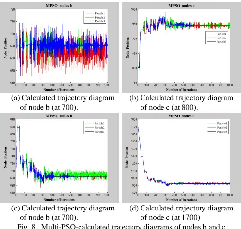
Fig. 8-(a) and 8-(c) show the trajectory diagram obtained when multi-PSO was used to calculate the fault curve of positions 1, 4 (Table 3) for node b.

Fig. 8-(b) and 8-(d) show the trajectory diagram obtained when multi-PSO was used to calculate the fault curve of positions 1, 4 (Table 3) for node c.

MPSO nodes b

Particle1 Particle2 Particle3 N o d e P o si ti o n

MPSO nodes c

N o d e P o si ti o n

Number of Iterations Particle1 Particle2 Particle3

(a) Calculated trajectory diagram (b) Calculated trajectory diagram of node b (at 700). of node c (at 800).

MPSO nodes b

MPSO nodes c

(c) Calculated trajectory diagram (d) Calculated trajectory diagram of node b (at 700). of node c (at 1700). Fig. 8. Multi-PSO-calculated trajectory diagrams of nodes b and c.

Table 4 shows that during the optimization of the FTU fault curve by using the standard PSO algorithm, the initial positions of nodes b and c are 700 and 800; this table indicates that after the iterations, the positions of nodes c and b obtained using the minimum area method are close to their initial positions. The other initial positions are considerably different from the positions of nodes c and b obtained using the minimum area method. The reason for this is that node b influences node c when the standard PSO algorithm is used to optimize the FTU fault curve. The origin of node c moves left and right, leading to the iteration results of the node c position being virtually the same as those of the initial node c position. Thus, during the execution of the standard PSO algorithm, node c falls into local solutions, resulting in early convergence. This affects the optimization of the overall FTU fault curve.

(8)

obtained using the multi-PSO algorithm on any position on the FTU fault curve are close to the optimal node positions obtained using the minimum area method. Figs. 7 and 8 indicate that this solves the limitation of the standard PSO, which is likely to fall into local solutions and cause early convergence.

Table IV Node positions.

Particle Swarm

Initial Setting Standard PSO Multi-PSO Minimum Area

Method Node b

Position Position Node c Position Node b Position Node c Position Node b Position Node c Position Node b Node c Position Particle 1 Particle 2 Particle 3 700 700 700 800 800 800 667.5039 683.4396 663.8100 799.0323 805.6277 804.4750 679.8318 690.9427 689.7829 943.5174 954.9361

944.7297 686.5731 931.8637 Particle 1 Particle 2 Particle 3 1,600 1,600 1,600 1,700 1,700 1,700 777.2 766.8 770.2 1,701.0 1,702.1 1,711.9 688.8 685.0 690.2 960.4 966.1 968.2

686.5731 931.8637

Particle 1 Particle 2 Particle 3 1,100 1,100 1,100 1,300 1,300 1,300 729.4 730.3 729.3 1,303.5 1,301.6 1,303.5 685.7 686.2 691.8 948.6 941.1 947.4

686.5731 931.8637

Particle 1 Particle 2 Particle 3 700 700 700 1,700 1,700 1,700 767.6984 757.6785 750.2963 1,581.7 1,587.1 1,577.6 684.1487 692.6748 684.8333 936.4 932.7 940.9

686.5731 931.8637

Table 5 shows that after the various node positions were calculated, the total jagged area obtained using multi-PSO is considerably smaller than that obtained using standard PSO. The values of the total jagged areas tend to converge and are close to the value of the total jagged area obtained using the minimum area algorithm. Thus, the multi-PSO algorithm has excellent global search and local convergence for nodes at diverse positions, improving the early convergence limitation of the standard PSO algorithm. After the jagged curve is calculated using the multi-PSO algorithm, the positions of the nodes on the jagged curve are adjusted. This adjustment results in the jagged curve exhibiting a relatively smooth and curved outline, achieving the required upstream-downstream protection coordination.

Table V

Comparison of the total jagged area.

Particle Swarm

Initial Position of Node b

Initial Position of Node c

Total Area of Initial Position Total Area With Standard PSO Total Area With Multi-PSO Total Area With Minimum Area Method Particle 1 Particle 2 Particle 3 700 700 700 800 800 800 2.1422 2.1422 2.1422 2.0674 2.0637 2.0670 2.0042 2.0043

2.0048 2.0036

Particle 1 Particle 2 Particle 3 1,600 1,600 1,600 1,700 1,700 1,700 3.4091 3.4091 3.4091 2.5140 2.5141 2.5057 2.0060 2.0058

2.0045 2.0036

Particle 1 Particle 2 Particle 3 1,100 1,100 1,100 1,300 1,300 1,300 2.7322 2.7322 2.7322 2.1927 2.1922 2.1924 2.0043 2.0053

2.0046 2.0036

Particle 1 Particle 2 Particle 3 700 700 700 1,700 1,700 1,700 2.5608 2.5608 2.5608 2.4142 2.4147 2.4286 2.0036 2.0046

2.0038 2.0036

VI. CONCLUSION

During the process of isolating feeder faults, the insufficient hardware computing power of FTUs necessitates using the TCC method to calculate fault curves, which results in jagged curves and considerably high detection errors. In this study, a multi-PSO algorithm was used to improve the excessive flagging and failure to flag caused by the rule-of-thumb methods currently used by Taipower. First, mathematical optimization is conducted to establish a mathematical model for optimizing a set points on the TCC. The objective function is the minimized curve area, and the constraints are that the set points must be within the interval between the fuse complete melting curve and the FCB fault curve and that the time interval between the FTU fault curve FCB fault curve must be at least

20% of the pu time value. The simulation results indicate that the multi-PSO algorithm can improve the early convergence problems encountered in the standard PSO algorithm. Next, the jagged curves formed by nodes were simulated at various positions. After the multi-PSO algorithm is executed to calculate the jagged curve and the node positions on the jagged curve are adjusted, the resulting jagged area is close to the moved nodes. This results in the jagged curve exhibiting relatively smooth and curved outlines, achieving the required upstream-downstream protection coordination. This substantially reduces malfunctions or erroneous nonoperation in the breakers. After 2 years of testing, the proposed method is determined to be able to effectively improve misjudgment of faults on the distribution feeders by FTUs. This increases the success rate of the expert system (FDIR).

ACKNOWLEDGMENT

The authors gratefully thank the assistance from the distribution department of Taipower to provide the valuable data and the assistance of on-site testing as well as excellent discussion. The financial support to this work by the Taipower is also highly appreciated.

REFERENCES

[1] M. Meiqin, J. Meihong, D. Wei and L. Chang, “Multi-objective Economic Dispatch Model for A Microgrid Considering Reliability,”

IEEE Power Electronics for Distributed Generation Systems (PEDG) on International Symposium, 2010, pp.993-998.

[2] Qi Kang, MengChu Zhou, Jing An, Qidi Wu, “Swarm Intelligence Approaches to Optimal Power Flow Problem With Distributed Generator Failures in Power Networks”, IEEE Trans. Power on Automation Science and Engineering, vol. 10, no. 2, pp. 344-353, April 2013.

[3] Mo N., Zou Z.Y., Chan K.W., Pong T.Y.G. , “Transient Stability Constrained Optimal Power Flow Using Particle Swarm Optimisation”,

IET Gener. Distrib., pp. 476-483, January 2007.

[4] Das T.K., Venayagamoorthy G.K., Aliyu U.O., “Bio-Inspired Algorithms for the Design of Multiple Optimal Power System Stabilizers: SPPSO and BFA”, IEEE Trans. Ind. Appl., vol. 44, no. 5, pp. 1445-1457, October 2008.

[5] Communications Systems Division, Taiwan Power Company. “Test Website for Calculating FTU Optimal Settings.” Taipower Operations, Taipei, 2009.

[6] Taiwan Power Company. “Distribution Technical Manual (25), Feeder Automation Engineering.” Taipower Operations, Taipei, 2009. [7] Taiwan Power Company, “IED Specifications.” Taipower Operations,

Taipei, 2009.

[8] Daneshyari M., Yen G.G., “Constrained Multiple-Swarm Particle Swarm Optimization Within a Cultural Framework”, IEEE Trans. on System,

Man, and Cybernetics- Part A: System and Humans, vol. 42, no. 2, pp. 475-490, March 2012.

[9] Yen G.G., Wen Fung Leong, “Dynamic Multiple Swarms in Multiobjective Particle Swarm Optimization”, IEEE Trans. on System,

Man, and Cybernetics- Part A: System and Humans, vol. 39, no. 4, pp. 890-911, July 2009.

[10] Jurgen Schlabbach, “Short-Circuit Currents”, The Institution of Electrical Engineers, London, United Kingdom, pp.1-96, 2005.

[11] Hadi Saadat, “Power System Analysis”, McGraw-Hill international Editions, pp. 353-459, 1999.

(9)

Ming-Yuan Cho(M’92) is with the Department of Electrical Engineering, National Kaohsiung University of Applied Sciences (KUAS), where he is currently a distinguished professor associated with the Dean of College of Electrical Engineering and Computer Science at KUAS. He has also served as the chairman of Department of Electrical Engineering at KUAS from August, 2000 to July, 2003. His research interests are smart grid, energy saving technologies and artificial intelligent algorithm for power system applications.

Shen-Wen Hsiao is currently pursuing the Ph.D. degree at the institute of electrical engineering in National Kaohsiung University of Applied Sciences, Taiwan. The past couple of years have been an exceedingly busy and challenging time for his study. His research interests are optimization, support vector machine and neural network in transmission and distribution system for power system applications.