Illumination Invariant Deep Learning for Hyperspectral Data

Learning for Hyperspectral Data

Lloyd Windrim

A thesis submitted in fulfillment of the requirements of the degree of

Doctor of Philosophy

Australian Centre for Field Robotics

School of Aerospace, Mechanical and Mechatronic Engineering The University of Sydney

I hereby declare that this submission is my own work and that, to the best of my knowledge and belief, it contains no material previously published or written by another person nor material which to a substantial extent has been accepted for the award of any other degree or diploma of the University or other institute of higher learning, except where due acknowledgement has been made in the text.

Lloyd Windrim

Motivated by the variability in hyperspectral images due to illumination and the diffi-culty in acquiring labelled data, this thesis proposes different approaches for learning illumination invariant feature representations and classification models for hyperspec-tral data captured outdoors, under natural sunlight. The approaches integrate domain knowledge into learning algorithms and hence does not rely on a priori knowledge

of atmospheric parameters, additional sensors or large amounts of labelled training data.

Hyperspectral sensors record rich semantic information from a scene, making them useful for robotics or remote sensing applications where perception systems are used to gain an understanding of the scene. Images recorded by hyperspectral sensors can, however, be affected to varying degrees by intrinsic factors relating to the sensor itself (keystone, smile, noise, particularly at the limits of the sensed spectral range) but also by extrinsic factors such as the way the scene is illuminated. The appearance of the scene in the image is tied to the incident illumination which is dependent on variables such as the position of the sun, geometry of the surface and the prevailing atmospheric conditions. Effects like shadows can make the appearance and spectral characteristics of identical materials to be significantly different. This degrades the performance of high-level algorithms that use hyperspectral data, such as those that do classification and clustering.

If sufficient training data is available, learning algorithms such as neural networks can capture variability in the scene appearance and be trained to compensate for it. Learning algorithms are advantageous for this task because they do not require

a priori knowledge of the prevailing atmospheric conditions or data from additional

sensors. Labelling of hyperspectral data is, however, difficult and time-consuming, so acquiring enough labelled samples for the learning algorithm to adequately capture the scene appearance is challenging. Hence, there is a need for the development of techniques that are invariant to the effects of illumination that do not require large amounts of labelled data.

In this thesis, an approach to learning a representation of hyperspectral data that is invariant to the effects of illumination is proposed. This approach combines a

physics-based model of the illumination process with an unsupervised deep learning algorithm, and thus requires no labelled data. Datasets that vary both temporally and spatially are used to compare the proposed approach to other similar state-of-the-art techniques. The results show that the learnt representation is more invariant to shadows in the image and to variations in brightness due to changes in the scene topography or position of the sun in the sky. The results also show that a supervised classifier can predict class labels more accurately and more consistently across time when images are represented using the proposed method.

Additionally, this thesis proposes methods to train supervised classification models to be more robust to variations in illumination where only limited amounts of la-belled data are available. The transfer of knowledge from well-lala-belled datasets to poorly labelled datasets for classification is investigated. A method is also proposed for enabling small amounts of labelled samples to capture the variability in spectra across the scene. These samples are then used to train a classifier to be robust to the variability in the data caused by variations in illumination. The results show that these approaches make convolutional neural network classifiers more robust and achieve better performance when there is limited labelled training data.

A case study is presented where a pipeline is proposed that incorporates the methods proposed in this thesis for learning robust feature representations and classification models. A scene is clustered using no labelled data. The results show that the pipeline groups the data into clusters that are consistent with the spatial distribution of the classes in the scene as determined from ground truth.

I would like to thank my supervisors Arman Melkumyan, Richard Murphy and Anna Chlingaryan for their invaluable guidance over the last few years. Between the three of you there was such a wide breadth of knowledge and I have always felt wiser after my discussions with you. Thank you for all of the advice you gave me - whether it was related to thesis work, research philosophy, careers or anything in general. A special thank you to my friend Rishi Ramakrishnan who has been my unofficial mentor since I was an undergraduate. You were the one who got me interested in the research topics I chose to pursue. I am infinitely grateful for the great many things I have learnt from you over the years, and for keeping me sane throughout the process (you were my go to for procrastination).

Thank you to my parents and sister for always pushing me, supporting me and check-ing up on my progress. It is thanks to you that I am where I am today. Thank you to Abbey for all of her love and support, and for helping me to maintain balance. Thank you to everyone at the Australian Centre for Field Robotics and Sydney Uni-versity. In particular, thank you to Andrew, Zach, Victor, Rishi, Tatsumi, Phil, Nader, Troy, Eric, Alex, Suchet, Jono, Steve and John for all of the lunches, coffee and discussions. I am also very grateful for all of the financial support and resources provided by the Rio Tinto Centre for Mining Automation, without which this work would not have been possible. Thank you to Steve Scheding and Salah Sukkarieh for your great leadership.

Thank you to the rest of my friends and family for all of the positive distractions. A special thank you to my original supervisor Juan Nieto for opening the doors to the world of academia to me. You took me on as your student and in a short amount of time instilled in me a great research philosophy.

Declaration i

Abstract ii

Acknowledgements iv

Contents v

List of Figures x

List of Tables xiv

List of Algorithms xv Nomenclature xvi Glossary xviii 1 Introduction 1 1.1 Motivation . . . 1 1.2 Contributions of Thesis . . . 6 1.3 Publications . . . 8 1.4 Structure of Thesis . . . 9

2 Background 11

2.1 Hyperspectral Sensing . . . 11

2.1.1 Classification . . . 13

2.1.2 Dimensionality Reduction . . . 16

2.2 Outdoor Illumination Model and Relighting . . . 17

2.2.1 Sources of Illumination . . . 17

2.2.2 Physics-Based Illumination Model . . . 19

2.2.3 Relighting . . . 19

2.3 Deep Learning . . . 20

2.3.1 Multi-layer Perceptron . . . 21

2.3.2 Autoencoder . . . 25

2.3.3 Convolutional Neural Network . . . 27

2.4 Literature Review . . . 30

2.4.1 Illumination Invariance . . . 31

2.4.2 Advancements in Convolutional Neural Networks . . . 40

2.4.3 Deep Learning Models for Hyperspectral Data . . . 41

2.4.4 Data augmentation . . . 45

2.4.5 Summary . . . 46

3 Datasets and Metrics 48 3.1 Datasets . . . 48

3.1.1 Sensors . . . 50

3.1.2 Dataset 1: Simulated USGS . . . 51

3.1.3 Dataset 2: X-rite panel . . . 53

3.1.4 Dataset 3: Great Hall (VNIR) . . . 54

3.1.5 Dataset 4: Great Hall (SWIR) . . . 55

3.1.6 Dataset 5: Mining timelapse . . . 56

3.1.7 Dataset 6: Mining . . . 57

3.1.9 Dataset 8: Gualtar timelapse . . . 60

3.1.10 Dataset 9: Pavia University . . . 60

3.1.11 Dataset 10: Kennedy Space Centre . . . 62

3.1.12 Dataset 11: Indian Pines . . . 62

3.1.13 Dataset 12: Salinas . . . 64

3.2 Metrics . . . 65

3.2.1 Fisher’s discriminant ratio . . . 65

3.2.2 Adjusted rand index . . . 66

3.2.3 Peak signal-to-noise ratio . . . 66

3.2.4 Percentage change in classification label . . . 67

3.2.5 F1 classification score . . . 68

3.2.6 Number of epochs . . . 68

4 Unsupervised Illumination Invariant Representation of Hyperspec-tral Data 70 4.1 Hyperspectral Stacked Autoencoders . . . 72

4.1.1 Cosine Spectral Angle Stacked Autoencoder . . . 73

4.1.2 Spectral Angle Stacked Autoencoder . . . 75

4.1.3 Spectral Information Divergence Stacked Autoencoder . . . . 76

4.2 Relit Spectral Angle Stacked Autoencoder . . . 77

4.2.1 Overview . . . 79

4.2.2 Autoencoder Framework . . . 81

4.2.3 Training . . . 81

4.2.4 Spectral Relighting . . . 82

4.3 Experimental Results . . . 87

4.3.1 Network Architecture and Parameters . . . 87

4.3.2 Evaluation of Hyperspectral Stacked Autoencoders . . . 88

4.3.3 Evaluation of RSA-SAE . . . 94

4.4 Discussion . . . 107

4.4.1 Evaluation of Hyperspectral Stacked Autoencoders . . . 108

4.4.2 Evaluation of RSA-SAE . . . 111

5 Supervised Classification of Hyperspectral Data with Limited

Train-ing Samples 117

5.1 CNN Architecture for Hyperspectral Classification . . . 119

5.2 Transfer Learning . . . 122

5.2.1 Datasets to use for pre-training . . . 127

5.2.2 Forming a composite dataset for pre-training . . . 128

5.2.3 Pre-training and fine-tuning a network . . . 130

5.3 Spectral Relighting Augmentation . . . 131

5.3.1 Augmenting Spectra . . . 132

5.3.2 Image Based Estimation of the Terrestrial Sunlight-Diffuse Sky-light Ratio . . . 134

5.4 Experimental Results . . . 138

5.4.1 Network Architecture and Parameters . . . 138

5.4.2 Evaluation of Transfer Learning . . . 140

5.4.3 Evaluation of Spectral Relighting Augmentation . . . 151

5.4.4 Analysis of the Learnt Filters . . . 162

5.5 Discussion . . . 166

5.5.1 Evaluation of Transfer Learning . . . 166

5.5.2 Evaluation of Spectral Relighting Augmentation . . . 169

5.5.3 Analysis of the Learnt Filters . . . 172

5.6 Summary . . . 173

6 Case Study: A Unified Pipeline 174 6.1 Problem Definition . . . 174

6.2 Pipeline . . . 176

6.2.1 Unsupervised Process . . . 177

6.2.2 Self-Supervised Process . . . 178

6.3 Results and Discussion . . . 179

6.3.1 Implementation Specifications . . . 179

6.3.2 Results . . . 179

6.3.3 Discussion . . . 183

7 Conclusions 187

7.1 Summary . . . 187 7.2 Contributions . . . 188 7.3 Future Work . . . 191

List of References 193

A Derivation of the CSA-SAE 214

A.1 Derivative of the Sigmoid Activation Function . . . 222

B Derivation of the SA-SAE 223

C Derivation of the SID-SAE 227

D Derivation of the relighting equations 231

D.1 Relighting with respect to diffuse skylight . . . 231 D.2 Relighting with respect to full terrestrial sunlight and diffuse skylight 232 D.3 Relighting with respect to a generalised illuminant . . . 233

1.1 Example of illumination variability in an RGB image. . . 3

1.2 Difficulty in labelling an image . . . 4

1.3 Use of spectrometer in the field . . . 5

2.1 Difference between RGB and hyperspectral sensor. . . 12

2.2 Hypercube. . . 13

2.3 The three sources of illumination in an outdoor scene. . . 18

2.4 Differences between sunlight and diffuse skylight. . . 18

2.5 Basic neural networks. . . 22

2.6 An example of a stacked autoencoder. . . 26

2.7 An example of a stacked DAE. . . 28

2.8 An example of a CNN architecture - AlexNet. . . 28

2.9 A 3×3 kernel filtering a 2D image to produce a feature map. . . 29

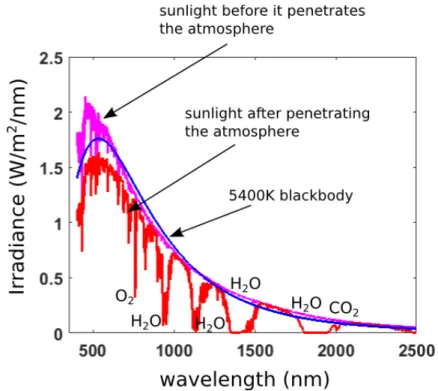
2.10 The effect of the atmosphere on the solar radiation spectrum. . . 34

3.1 Simulated USGS dataset. . . 52

3.2 The X-rite dataset. . . 53

3.3 Great Hall (VNIR) dataset. . . 54

3.4 Great Hall (SWIR) dataset. . . 55

3.5 Colour composite images from the mining timelapse dataset. . . 56

3.6 RGB images of the mine. . . 56

3.8 Mining dataset. . . 58

3.9 Gualtar steps dataset. . . 59

3.10 Gualtar timelapse dataset. . . 60

3.11 Colour composite images from the gualtar timelapse dataset. . . 61

3.12 Pavia Uni dataset. . . 62

3.13 KSC dataset. . . 63

3.14 Indian Pines dataset. . . 63

3.15 Salinas dataset. . . 64

4.1 Framework for training the RSA-SAE network. . . 80

4.2 Summary of process for training the RSA-SAE network. . . 86

4.3 Comparison of the representation power of different techniques. . . . 90

4.4 Comparison of clustering results. . . 91

4.5 Comparison of brightness invariance of different techniques. . . 92

4.6 Brightness invariance of low dimensional representation. . . 93

4.7 Comparison of illuminant invariance of different techniques. . . 94

4.8 Illuminant invariance of low dimensional representation. . . 95

4.9 Qualitative results from the Gualtar steps. . . 96

4.10 Feature vector results from the Gualtar steps. . . 100

4.11 Gualtar timelapse qualitative results. . . 102

4.12 Gualtar timelapse quantitative results. . . 103

4.13 Mineface qualitative results. . . 106

4.14 Comparison of sunlit, shadow and augmented spectra from mineface. 107 5.1 Simplified diagram of example CNN architecture used. . . 120

5.2 Impact of water absorption on spectra. . . 122

5.3 An example CNN filter convolving over a vegetation spectra. . . 123

5.4 The basic transfer learning process. . . 124

5.6 Candidate pairs along horizontal and vertical transects projected onto illumination and invariant axes. . . 137 5.7 Extracting Lsun/Lshadow. . . 139

5.8 Transfer learning results: different filter sizes. . . 142 5.9 Transfer learning results: pre-training verses training from scratch for

different numbers of training samples. . . 147 5.10 Transfer learning results: Mean percentage change in parameters from

initialisation to convergence. . . 148 5.11 Transfer learning results: pre-training versus training from scratch for

different architectures. . . 149 5.12 Transfer learning results: pre-training verses training from scratch for

a spectral-spatial network. . . 151 5.13 Spectral relighting augmentation quantitative classification results. . . 154 5.14 Spectral relighting augmentation qualitative Great Hall classification

results. . . 155 5.15 Spectral relighting augmentation qualitative mining timelapse

classifi-cation results. . . 155 5.16 Spectral relighting augmentation qualitative Gualtar steps

classifica-tion results. . . 156 5.17 Spectral relighting augmentation results: Classification score in shadow

and sunlight. . . 156 5.18 Spectral relighting augmentation results: Percentage of pixels that

changed label. . . 157 5.19 Spectral relighting augmentation results: Candidate pairs of sun-shadow

pixels. . . 157 5.20 Spectral relighting augmentation results: Automatic extraction ofLA/LA0.158

5.21 Spectral relighting augmentation results: Qualitative accuracy of spec-tra relighting. . . 158 5.22 Spectral relighting augmentation results: Reflectance verses DN. . . . 159 5.23 Spectral relighting augmentation results: Comparison of different

ar-chitectures. . . 159 5.24 Spectral relighting augmentation results: SVM and SAM. . . 160 5.25 Spectral relighting augmentation results: Spatial-spectral network. . . 161

5.26 Spectral relighting augmentation results: Different methods for ex-tracting the terrestrial sunlight-diffuse skylight ratio . . . 162 5.27 Filter analysis results: Visualisation of the first 10 filters of the first

layer. . . 163 5.28 Filter analysis results: First layer activation. . . 164 5.29 Filter analysis results: Third layer activation. . . 165 6.1 The mining 11:30 timelapse image with ground truth areas highlighted. 176 6.2 A flowchart summarising the pipeline for clustering. . . 178 6.3 Results from the different steps of the unsupervised process. . . 180 6.4 The result of clustering in the original reflectance space. . . 181 6.5 Images of the mineface captured at different times of the day but

as-signed categories with the same CNN. . . 182 6.6 Change in the F1 score for the different elements of the self-supervised

4.3 Quantitative results from the Gualtar steps and Great Hall. . . 98

4.4 Gualtar timelapse quantitative results. . . 103

4.5 Mineface quantitative results. . . 105

5.1 A selection of the most common, annotated hyperspectral datasets which are publicly available. . . 127

5.2 Classes and number of samples for Indian Pines. . . 128

5.3 Classes and number of samples for Salinas. . . 129

5.4 Classes and number of samples for Pavia University. . . 129

5.5 The classes chosen from each dataset to pre-train the composite CNNs. 144 5.6 Spectral relighting augmentation results: Quantitative form of the re-sults in Figure 5.26. . . 162

5.1 Procedure for pre-training a CNN and then transferring the knowledge learnt - by fine-tuning for a new task. . . 130 5.2 Augmenting a batch of spectra for training the CNN.U andB represent

List of Symbols

a(_il) activation of neuron i in layer l

b(_jl) bias of neuron j in layerl+1

Cml number of rows in each kernel in the l-th convolutional layer

Cnl number of columns in each kernel in the l-th convolutional layer

Cdl number of dimensions in each kernel in the l-th convolutional layer

E cost function for neural network

Eind indirect illumination irradiance spectrum (function of wavelength)

Esky diffuse skylight irradiance spectrum (function of wavelength)

Esun extraterrestrial sunlight irradiance spectrum (function of wavelength)

Esunτ terrestrial sunlight irradiance spectrum (function of wavelength)

f(·) activation function

K number of spectral channels

L radiance or digital number of spectra (function of wavelength)

l layer number of a neural network

V line-of-sight visibility between region and sun

W_ji(l) the weight connecting neuron i in layer l with neuronj in layer l+1

X log-chromaticity

xi feature value i of the input to the neural network

yi feature value i of the target of the neural network

z_i(l) weighted sum of neurons in layer (l-1) and the bias term going into

the i-th neuron in layer l

α learning rate

Γ sky (or view) factor

ω direction of the illumination invariant axis in log-chromaticity space

ρ albedo (function of wavelength)

θ angle between the surface normal and vector towards the sun

List of Acronyms

ARI adjusted rand index

AVIRIS airborne visible/infrared imaging spectrometer

CNN convolutional neural network

CRF conditional random field

CSA-SAE cosine spectral angle-stacked autoencoder

DAE denoising autoencoder

DN digital number

FA factor analysis

GP Gaussian process

GPS global positioning system

GPU graphics processing unit

IARR internal average relative reflectance

ICA independent component analysis

ILSVRC ImageNet large scale visual recognition challenge

KNN k-nearest-neighbour

KSC Kennedy space station

LDA linear discriminant analysis

LiDAR light detection and ranging (also commonly known as a ‘laser range scanner’)

LLE local linear embedding

MLP multi-layer perceptron

MSE mean squared error

PCA principal component analysis

PSNR peak signal-to-noise ratio ReLU rectified linear unit

ROSIS-3 reflective optics system imaging spectrometer RSA-SAE relit spectral angle-stacked autoencoder SA-SAE spectral angle-stacked autoencoder

SAE stacked autoencoder

SAM spectral angle mapper

SID spectral information divergence

SID-SAE spectral information divergence-stacked autoencoder SSE-SAE sum of squared errors-stacked autoencoder

SWIR short-wave infrared

SVM support vector machine

USGS United States geological survey

VIS visible

Autoencoder: A type of neural network which learns to reconstruct an input in the

output layer.

Convolutional Neural Network: A type of neural network which learns localised

kernels which convolve over the data.

Diffuse: A material that reflects light uniformly in all directions. Also called

Lam-bertian.

Diffuse Skylight: Extraterrestrial sunlight that has been scattered by particles in

the atmosphere. Predominantly blue in colour.

Digital Number: The units of a pixels intensity as measured by a sensor. Incident Illumination: The light that illuminates a region in the scene.

Neural Network: A computational network of mathematical units capable of

learn-ing a mapplearn-ing from an input to an output. Related to the field of deep learnlearn-ing.

Radiometric Normalisation: The process of converting the digital number of each

pixel to reflectance.

Sky Factor: Proportion of the sky dome hemisphere that is visible from a region in

the scene.

Terrestrial Sunlight: Extraterrestrial sunlight that has not been scattered by

Introduction

The use of hyperspectral data in supervised applications is constrained by the lack of labelled training data. Thus, the aim of this thesis is to develop illumination invariant representations and classification models for outdoor hyperspectral data that use limited or no labelled training samples. When collected in the outdoor environment, where the light source is the sun, much of the variability in hyperspectral data spanning the visible to short-wave infrared (SWIR) wavelengths is related to how the scene is illuminated and collecting and annotating enough data to capture this variability is difficult. Through the use of learning algorithms that leverage models of the physical processes involved with scene illumination, this thesis presents an approach to robustly representing and classifying hyperspectral data acquired under natural light with little to no annotated training data.

1.1

Motivation

Sensors which perceive the environment provide a means in which machines can quan-tify and mimic human understanding of the physical world. The perceptual data col-lected from sensors on-board robots and remote-sensing platforms provide a wealth of information which can be harvested and interpreted in order to carry out high-level processes such as classification (e.g. Camps-Valls et al. (2014)), odometry (e.g. Nistér

et al. (2004)), planning (e.g. Baltzakis et al. (2003)), mapping (e.g. Se et al. (2002)), detection (e.g. Ren et al. (2015)) and recognition (e.g. Turk and Pentland (1991)). Imaging sensors in particular have received considerable attention in the develop-ment of these platforms due to their ability to non-destructively capture information at high spatial resolution and their ability to work from a variety of viewing distances and under a variety of different environmental conditions (e.g. rain). Hyperspec-tral sensors are a particularly powerful variety of imaging sensor that are capable of measuring the spectral reflectance of objects in numerous, contiguous band-passes in the visible to SWIR range. Unlike multispectral sensors which measure reflectance in a small number of broad, discontiguous bands of variable width, hyperspectral sensors capture the entire spectral curve, seamlessly across the observed range. This makes it possible to resolve the shape, intensity and wavelength location of absorp-tions within the spectrum that are relevant to a broad range of quantitative tasks including geological mapping, agriculture and defence (Schowengerdt, 2007).

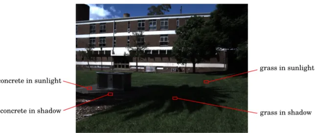
A major problem with using an imaging system operating outdoors, in particular a hyperspectral imaging system, is that the appearance of the scene is highly variable (Ramakrishnan, 2016). When capturing the appearance of a scene, variations (e.g. in brightness) are translated to the image resulting in degradations in the performance of high-level tasks using the image data (Corke et al., 2013). This is because objects and materials that are intrinsically similar can appear to be differently in the image and objects and materials that are intrinsically different can appear to be similarly in the image (Figure 1.1). The appearance of a scene is determined largely by the ways in which light interacts with the environment. Consequently, along with non-Lambertian factors, one of the largest sources of variability in scene appearance is related to the variability of the incident illumination.

The appearance of the scene as measured by a camera is based on how the scene reflects incoming light, that is, the incident illumination. When light is emitted from the sun it transmits through the atmosphere and is absorbed and scattered across certain wavelengths by atmospheric gasses, water and other particles (Schowengerdt, 2007). This modifies the colour temperature and intensity of the spectrum of incident

Figure 1.1– Example of illumination variability in an RGB image. Scene constituents that are semantically similar appear differently under shadow and sunlight (e.g. the grass), and constituents that are semantically different appear similarly in shadow (e.g. the grass and concrete).

light based on the ambient atmospheric composition. Hence, obtaining measurements under consistent conditions over long periods of time is difficult due to the variability in the primary light source illuminating the scene (i.e. sunlight).

Additionally, there are factors which alter how the incident light illuminates the scene in a single image. The spectrum of the incident light source is modified by the geometry of the scene (Schowengerdt, 2007). The angle at which the illuminant strikes the surface effects the intensity at which it is reflected back (Hapke, 1981). Parts of the scene may also occlude other regions of the scene from the primary light source. However, these occluded regions may still be illuminated by indirect sources of light, such as rays from the primary source that are reflected off of the sky and other materials in the scene. This phenomenon results in shadows. The indirect incident illuminant bears the wavelength-intensity distribution of light of the materials from which it is reflected and hence differs significantly from the primary light source. This effect is also possible when there are clouds occluding the primary light source. The amount of sky visible to the surface influences how much indirect skylight it is illuminated by.

(a)Almonds in a tree (Bargoti and Un-derwood, 2017).

(b)A mine face containing Martite and Shale (Murphy et al., 2012).

Figure 1.2– It is difficult to label the constituents of both of these images.

the azimuth and elevation of the sun, which can vary over time, the geometry of the scene, which varies across a single image, and the material properties of elements of the scene. Estimating material properties is valuable for use in high-level algorithms, however, isolating them from the other factors of variation remains an ill-posed prob-lem due to the number of unknown variables and complex ways in which they interact. If high-level algorithms using hyperspectral data are to work reliably in the outdoors, it is important to find representations and classification models that are robust to these complex interactions.

As the development of learning algorithms moves forward at a rapid pace, a trend is emerging in their application to image data. There is a strong reliance on using large datasets to teach learning algorithms to solve problems. For example, very

Figure 1.3– Use of a spectrometer in the field to obtain ground truth information.

good classification results can be achieved by training on a very large dataset which captures all of the variability in the data (e.g. Krizhevsky and Hinton (2012), Szegedy et al. (2015)). In doing so, it is less tempting to incorporate domain knowledge into state-of-the-art techniques, for example, physics-based models that have been developed over many years which mathematically model the interactions of light with the environment (e.g. Hapke (1981)). The strong reliance on large datasets is only feasible when large labelled datasets are available for learning and unfortunately for applications which use hyperspectral data, labelled data is limited due to the difficulty in acquiring it.

Once captured, there are multiple ways of assigning labels to hyperspectral data (i.e. annotating pixel data). One approach is by visually inspecting RGB colour imagery, individual bands or false-colour imagery constructed from other wavelengths beyond the visible range and then manually labelling regions of pixels. In many scenarios, particularly when there is a high degree of variation in illumination, this can be challenging because different materials can appear similar (Figure 1.1). For example, in an agriculture context, labelling green apples, avocados or almonds in a tree is problematic due to their similar appearance to leaves, both in colour and texture (Figure 1.2a). Another example is in an open pit mining operation where different materials can appear very similar (Murphy et al., 2014a). In Figure 1.2b, it is very difficult to distinguish between the shale region and the martite region of the mine face. An alternative to labelling regions of pixels by inspection of the image is to look at the spectral information of individual pixels, and have an expert annotate them. The spectral information is much more informative of the material’s class, but it is

challenging and time-consuming to label individual pixels. In reality, this is because the pixel spectra from the image are often affected by illumination, noise and spectral mixing among other things. The spectra that are the most unrecognisable, such as the ones in shadow, can be difficult to label. However, these examples are necessary to train the classifier to be robust to the sorts of effects expected in the image. For these reasons it is usually necessary to take a field spectrometer into the environment (Figure 1.3) and measure the spectra of individual targets at high spectral resolution, and then tag the location or target so that it can be matched to the image. The targets can be artificially illuminated and spectra collected are generally less noisy than there image counterparts making it easier to label, however, collecting the readings is extremely laborious because of the difficulties in aligning the spatial scale of the samples with the spatial scale of the image, co-locating the measurements with pixels in the image and collecting a large number of measurements at the sufficient spatial resolution. In environments such mine pits, interacting with the scene can also be hazardous with the possibility of rock falls, explosives and heavy machinery in the environment. In summary, annotating hyperspectral data is difficult, thus classifiers and feature learners are often limited to using small amounts of labelled training data that do not accurately capture the variability of the scene. If the labelled data does not capture the large and complex variability in the outdoor scene, then it cannot be modelled by learning algorithms for applications which use hyperspectral data. Because of the difficulty in labelling hyperspectral data for training, there is a need to develop methods which are robust to large variations in hyperspectral data due to illumination that do not require a large amount of labelled data.

1.2

Contributions of Thesis

In this thesis, an approach is proposed for learning illumination invariant representa-tions and classification models for outdoor hyperspectral data. The approach lever-age’s domain knowledge in the form of physics-based models, and learns the elements to the problem that are unknown. By integrating domain knowledge into learning

al-gorithms (specifically, deep learning alal-gorithms), fewer labelled samples are required for learning, but the representations and classification models can still account for large amounts of variation in the data. Specifically, the illumination effects targeted are the influence of the geometry of the surface with respect to the sun and sky on the incident illumination, including variations in brightness and shadows caused by occlusions from the primary light source.

The specific contributions are:

• A set of unsupervised approaches to learning feature representations specifically

designed for hyperspectral data. The approaches use remote sensing methods to improve a deep learning technique, and the representations are designed to be invariant to variations in the intensity (i.e. brightness) of the incident illuminant and improve performance when scenes have a variable surface geometry. These techniques are useful for dimensionality reduction or feature extraction.

• An extended unsupervised approach to learning a low-dimensional,

illumina-tion invariant feature representaillumina-tion of hyperspectral data. This representaillumina-tion retains the discriminative information of the original spectra, but is also invari-ant to shadows as well as illumination intensity effects. Hence, materials in an image that are the same will appear the same, regardless of the illumination effects. The technique requires no labelled data, a priori knowledge or

addi-tional sensors and the representation is useful for classification, clustering or any high-level task where robustness to the illumination is a desirable property.

• A transfer learning scheme for utilising training samples from well-labelled

hy-perspectral images in order to pre-train a classifier for better performance on poorly labelled images. This is useful for learning better spectral features when there are limited labelled training samples available. The pre-trained features are also faster to train. Using this scheme, it is possible to transfer knowledge from airborne datasets, of which there exist well-labelled, public datasets, to field-based datasets, which typically must be labelled from scratch.

• An image-based approach for estimating the terrestrial sunlight-diffuse skylight

ratio. This is important for spectral relighting (e.g. Marschner and Greenberg (1997)), which involves altering the appearance of an image such that it is illuminated differently. Relighting is used heavily in the context of this thesis.

• A relighting-based approach to learning a robust classification model using

lim-ited labelled training data. This classification model can predict labels for each pixel in a hyperspectral image, given a training set where the labels have poor spatial coverage of the scene. Samples acquired from localised, sunlit regions can train the classifier to accurately predict labels for regions with large variations in geometric orientation and regions in shadow.

1.3

Publications

The work in this thesis has led to the following publications:

• Lloyd Windrim, Arman Melkumyan, Richard Murphy, Anna Chlingaryan and

Juan Nieto. Unsupervised Feature Learning for Illumination Robustness. In

Proceedings of the International Conference on Image Processing, pages

4453-4457, IEEE, 2016. - This paper presents one of the unsupervised approaches proposed in Chapter 4 for learning feature representations specifically for hy-perspectral data that are invariant to the illumination intensity.

• Lloyd Windrim, Rishi Ramakrishnan, Arman Melkumyan and Richard Murphy.

A Physics-based Deep Learning Approach to Shadow Invariant Representations of Hyperspectral Images. InTransactions on Image Processing

27.2(2018):665-677, IEEE. - This paper extends the unsupervised approach proposed in Chap-ter 4 for learning hyperspectral feature representations that are invariant to both shadows and the illumination intensity.

• Lloyd Windrim, Rishi Ramakrishnan, Arman Melkumyan and Richard Murphy.

Hyperspectral CNN classification with Limited Training Samples. In Proceed-ings of the British Machine Vision Conference, pages 2.1-2.12, BMVA Press,

2017. - This paper presents the image-based approach to extracting the ter-restrial sunlight-diffuse skylight ratio as well as the relighting-based approach to learning a robust hyperspectral classification model when there is limited labelled training samples, proposed in Chapter 5.

• Lloyd Windrim, Arman Melkumyan, Richard Murphy, Anna Chlingaryan and

Rishi Ramakrishnan. Pretraining for Hyperspectral Convolutional Neural Net-work Classification. InTransactions on Geoscience and Remote Sensing, IEEE.

Accepted for inclusion in a future issue. Pre-print available as of 03 January 2018. - This paper presents the transfer learning scheme proposed in Chapter 5.

1.4

Structure of Thesis

This thesis is structured as follows:

Chapter 2 introduces hyperspectral sensing, the outdoor illumination model and

associated relighting equations and deep learning, followed by an overview of the relevant literature. The literature covered includes how illumination invariance has been approached using methods from the fields of computer vision, remote-sensing, multi-modal sensing and statistical learning, with a focus on approaches for hyper-spectral imagery. The literature tracking the progress of the convolutional neural network (CNN) is presented, along with a review of how deep learning has been utilised for hyperspectral applications. Finally, the use of data augmentation in ma-chine learning is briefly reviewed.

Chapter 3presents the datasets and evaluation metrics used throughout the thesis. Chapter 4 proposes unsupervised approaches to learning low-dimensional,

illumi-nation invariant feature representations for hyperspectral images. The approaches are extensively evaluated and the results and their implications are presented and analysed.

Chapter 5proposes a transfer learning scheme, image-based approach to estimating

learning robust hyperspectral classification models. This is for the scenario where there is limited labelled training data. The results of rigorous evaluation of these approaches are presented and analysed.

Chapter 6 develops a pipeline for a case study which utilises the proposed

unsuper-vised feature representation and robust classification model to cluster a hyperspectral image without using any labelled data. The performance of the pipeline is discussed.

Background

This chapter presents an overview of the theory most relevant to this thesis, followed by a summary of the literature. The relevant theory includes the basic principles of hyperspectral imagery, the illumination model and relighting that is used throughout this thesis, and deep learning, including the workings of an autoencoder and CNN. The literature addressing the problem of variability in illumination is reviewed, fol-lowed by the progression of deep learning and how it has been used for hyperspectral applications.

2.1

Hyperspectral Sensing

A digital RGB camera captures a high spatial resolution image over only three chan-nels, where each channel consists of an integration of the incident light over many wavelengths using a wide-band filter. Conversely, hyperspectral sensors capture high spatial resolution images with numerous channels (tens to hundreds) each covering a narrow range of wavelengths (Figure 2.1). Each pixel in a hyperspectral image contains the spectrum of the material it captures across the visible, near infrared and SWIR portions of the electromagnetic spectrum (e.g. in the range 400 nm to 2500 nm). Hence, each pixel spectrum provides a more detailed measurement of the reflectance behaviour of a material. Because reflectance is measured across narrow

(a)RGB sensor response. (b) Hyperspectral sensor response.

Figure 2.1 – An example of the differences between the sensor response of an RGB

camera and a hyperspectral camera in terms of the width and number of filters.

intervals of wavelength, subtle changes in reflectance can be detected that would be impossible to pick up with an RGB camera.

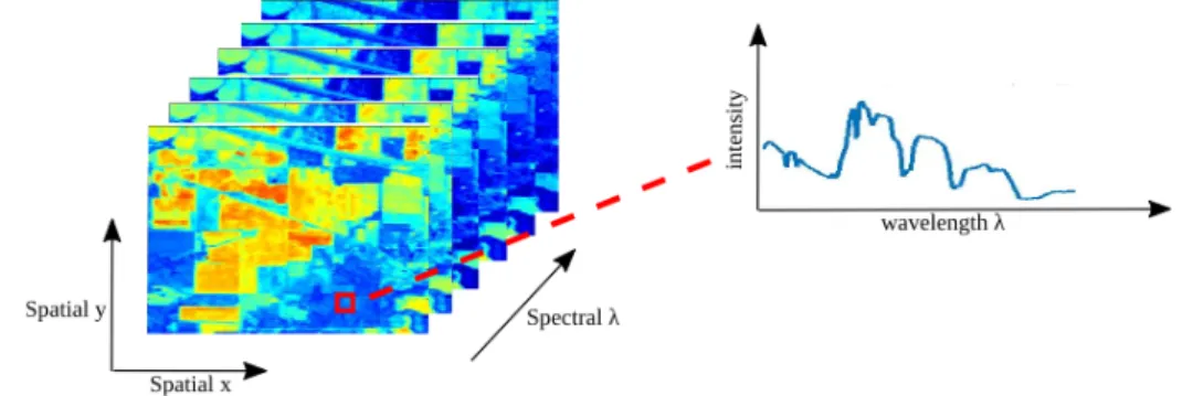
A hyperspectral image can be conceptualised as a cube, with two dimensions attribut-ing to the x and y dimensions of the scene and the third dimension formed by many

different wavelengths sequentially stacked one upon the other (Figure 2.2).

Hyperspectral images are typically acquired from sensors on-board airborne platforms such as aircraft and balloons and more recently data has been acquired from field-based platforms such as ground-field-based systems and robots. The higher the altitude of the sensor, the larger the area of ground described by each pixel is and thus the easier it is acquire scans with greater swath. However, as the pixel size increases, the spatial resolution decreases. If multiple spectrally distinct materials present in the scene are mixed together in a pattern that is too fine to be resolved by the spatial resolution of the sensor, then the pixels of the cube will be a composite (sum) of the reflectance signals from all of these materials. This process is called spectral mixing (Bioucas-dias et al., 2012; Mustard and Pieters, 1987). It is particularly prominent in hyperspectral data collected from airborne or spaceborne platforms because of the larger pixel sizes. There are also numerous ways in which environmental factors can affect the signal detected by hyperspectral sensors including the atmospheric conditions, the geometry of the scene and the season.

Figure 2.2 – A hyperspectral image can be conceptualised as a hypercube with two spatial dimensions and a spectral dimension.

Due to the high spatial and spectral resolution of hyperspectral images, it is possi-ble to identify surface materials from a scene through an analysis of their diagnostic spectral features. These diagnostic spectral absorption features appear due to pro-cesses relating to the chemical and structural composition of each material. This allows hyperspectral cameras to be used in many diverse applications such as food safety (Elmasry et al., 2012; Feng and Sun, 2012), military surveillance (Eismann et al., 1996; Stein et al., 2001; Yuen and Richardson, 2010), medical imaging (Lu and Fei, 2014), environmental monitoring (Adam et al., 2010; Govender et al., 2007), geological mapping (Murphy et al., 2012; Van der Meer et al., 2017) and precision agriculture (Haboudane et al., 2002).

2.1.1

Classification

Using classification algorithms, it is possible to automate the process of surface ma-terial identification of a scene from a hyperspectral image (Camps-Valls et al., 2014). The advantage of hyperspectral imagery is that each pixel contains sufficient informa-tion so that it is possible to classify a scene at the pixel level using these algorithms. There are a number of ways in which this is typically done.

One way is to build up a library of reference spectra, ideally collected under laboratory conditions using a non-imaging spectrometer. If the library contains several entries per class, then the pixel spectra in an image can be matched to the most similar entry in this library (Murphy et al., 2012). This determines its class. There are

many ways to match the spectra to the reference library, but the most common way is the spectral angle mapper (SAM) (Kruse et al., 1993; Yuhas et al., 1992). SAM computes the inverse cosine of the normalised dot product between the target spectra and all reference spectra in the library. A pixel is assigned the class of a reference spectra if it lies within a certain angular threshold (normally expressed in radians). Alternatively, a spectrum is assigned the class of the reference spectrum with which it has the smallest angle. The advantage of SAM is that it is robust to scaler multiples of the spectra that are constant across the wavelength, which can occur due to differences in brightness (Hecker et al., 2008).

Another approach is to collect training spectra from the image being examined, either as pixels in the image or samples collected from the scene that are scanned separately, annotate them and train a supervised classification model which can be used for inference. There are many methods for training a classification model, including a support vector machine (SVM) (Melgani and Bruzzone, 2004), k-nearest-neighbour (KNN) (Yang et al., 2010), Gaussian process (GP) (Schneider et al., 2010), decision tree (Ham et al., 2005) and neural networks (Ratle et al., 2009). Once the model has been trained to sufficiently minimise a loss function using enough samples to capture the variability of each class in the training set, the model can be used to predict the class label of new data drawn from the same distribution as the training data. Typically, to use the second approach, a small fraction of the pixels from each class in the scene to be classified are annotated and used to train the classifier. Then, predictions for the rest of the pixels in the image are computed using the classifier. The classifier requires each input pixel be described by a set of features. Features are the way in which the hyperspectral data are represented. The goal of the features is to make high-level tasks such as classification more efficient by maximising the separation between classes. It is possible to simply use the intensity or reflectance at each wavelength as the feature space. However, this is very simplistic and can often lead to problems with overfitting due to the dimensionality of the data (Bishop, 2006). Also, there is a lot of redundancy in this representation of the data due to the high degree of correlation between the channels (Demarchi et al., 2014). Traditionally,

it has been popular to use hand-crafted features which are designed using domain knowledge of the data. For example, layers of clay are mapped on a mine face using the width and depth of spectral absorption features at 2200 nm (Murphy et al., 2014a). It is often difficult, time-consuming and requires sufficient expertise to hand-craft these features, which is why an alternative approach is to use feature learning. Feature learning is an autonomous means of extracting features from the data. Methods for learning features can be supervised such as linear discriminant analysis (LDA) (Du, 2007) and kernel methods (Kuo et al., 2009). There are also unsupervised methods such as principal component analysis (PCA) (Cheriyadat and Bruce, 2003; Rodarmel and Shan, 2002) or independent component analysis (ICA) (Chiang et al., 2000). As an alternative to feature extraction, there are also feature selection techniques which find a subset of bands to use as features which optimise some criteria, such as class separation (Backer et al., 2005). Dimensionality reduction techniques (e.g. PCA) can be interpreted as feature extraction/selection methods as they are finding an abstraction of the raw data that is useful for classification.

Many of the hyperspectral classifiers mentioned above only use spectral information. However, many modern classification techniques also use the spatial dimension of the hyperspectral image. The spatial dimension provides contextual information about a pixel, which is usually correlated with its material class. A variety of approaches to spectral-spatial classification have been proposed. Some approaches combine morpho-logical features with spectral vectors (Fauvel et al., 2012, 2008). Other approaches use segmentation to spatially regularise a pixel-wise classification map. In Tara-balka et al. (2009), segmentation using partial clustering is combined with a spectral SVM classifier using majority voting. Similarly, watershed segmentation was used in Tarabalka et al. (2010). The classification maps obtained using spectral-spatial clas-sification methods are usually more homogeneous than those obtained from purely spectral-based methods.

2.1.2

Dimensionality Reduction

Dimensionality reduction is the statistical process of reducing the number of dimen-sions (or variables) required to describe a dataset. Hyperspectral datasets are of high dimensionality as the reflectance at each wavelength for a single pixel can be inter-preted as a separate dimension. The high dimensionality of hyperspectral data is linked to problems such as the curse of dimensionality (Donoho et al., 2000; Hughes, 1968; Lee and Landgrebe, 1993). With more dimensions, exponentially more data points are required to accurately represent the data’s distribution. Hence, a low ratio between the number of data points and the number of dimensions may limit many algorithms from working well where the data has a large number of dimensions. Most of the mass of a high dimensional multivariate Gaussian distribution is near its edges. Thus, many algorithms designed around an intuitive idea of ‘distance’ in two or three dimensional space, cease to work at higher dimensions, where those intuitions no longer hold. Other problems with having a high number of dimensions are the high storage requirements for the data and slow processing speeds (Bioucas-dias et al., 2012). For these reasons, many algorithms perform poorly when the data has too many dimensions due to the increased complexity of the task (Pal and Foody, 2010). Hyperdimensionality also makes it difficult to visualise the data without advanced software tools. As previously mentioned, because proximal wavelengths in hyper-spectral data are often highly correlated, there can be redundant information in the datacube. Therefore, it makes sense to reduce the number of dimensions in the data without loss of information.

The goal of dimensionality reduction is to compress the data whilst preserving all of its relevant information. As these criteria are also important for finding features, there is significant overlap in the techniques used for feature extraction/selection and dimensionality reduction. For this reason, many of the papers proposing dimension-ality techniques for hyperspectral data use a classification application as a means of evaluating them. Besides the basic techniques (e.g. PCA, factor analysis (FA) and ICA) there are many dimensionality reduction techniques that have been appropri-ated for use with hyperspectral data, such as local linear embedding (LLE) (Chen and

Qian, 2007; Han and Goodenough, 2005; Kim and Finkel, 2003), ISOMAP (Guangjun, Dong Yongsheng and Song, 2007; Sun et al., 2014) and Laplacian eigenmaps (Qian and Chen, 2007). Approaches also exist for dimensionality reduction of spectral-spatial features (Zhang et al., 2013). The need for reducing the dimensionality of hyperspectral data motivates the development of low-dimensional representations.

2.2

Outdoor Illumination Model and Relighting

Many of the techniques proposed in this thesis incorporate a model describing pro-cesses of illumination into deep neural networks. The model is described in this sec-tion. Firstly, the illumination sources assumed to be present in an outdoor scene are described. Then, the outdoor illumination model from which the relighting equations can be derived is explained.

2.2.1

Sources of Illumination

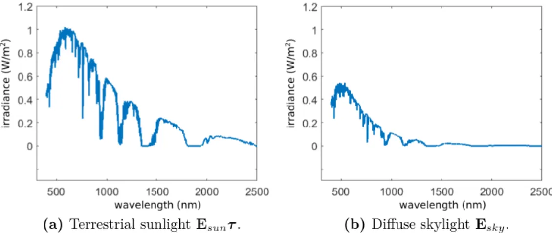
An outdoor scene has several sources of illumination, with the two most dominant sources being direct terrestrial sunlight and diffuse skylight (Gijsenij et al., 2012; Sato and Ikeuchi, 1995). The terrestrial sunlight source consists of the extraterres-trial light emitted from the sun that passes through earth’s atmosphere. The light takes on a spherical pattern when it is first emitted, but by the time it reaches earth it has travelled such a long distance that is can be considered a parallel light source (Schowengerdt, 2007). When the sunlight passes through the atmosphere, it is absorbed and scattered across specific ranges of wavelengths. The proportion of light that penetrates through the atmosphere and reaches the earth’s surface (called the solar path transmittance (Schowengerdt, 2007)) is wavelength dependent and ex-tremely variable. This is the terrestrial sunlight. The diffuse skylight occurs due to the Rayleigh scattering of light by particles that are smaller than the wavelength of the visible light. This results in blue light being preferably scattered (during daylight hours). By assuming consistent cloud coverage, the sky is considered to be a dome,

i

E

τ

j

E

E

Figure 2.3 – The three sources of illumination assumed to be present in an outdoor

scene, illuminating a region i. They are the terrestral sunlight E_sunτ, the diffuse skylightEsky and the indirect illumination Eindfrom the regionj.

(a)Terrestrial sunlightEsunτ. (b) Diffuse skylightEsky.

Figure 2.4 – Example of differences in intensity and spectral power distribution of

terrestrial sunlight and diffuse skylight as simulated by an atmospheric modeller (Gueymard, 2001).

and the diffuse skylight is modelled as a hemispherical light source (Sato and Ikeuchi, 1995). The intensity and spectral power distribution of the terrestrial sunlight differs significantly from the diffuse skylight, as seen in the example in Figure 2.4. Additional to these sources of illumination, there is indirect illumination. Light that is reflected off of surfaces in the scene can illuminate other surfaces, but with a much weaker intensity. The sources of illumination in outdoor scenes are shown in Figure 2.3.

2.2.2

Physics-Based Illumination Model

The following outdoor illumination model (Ramakrishnan, 2016) for the radiance of spectra reflected from a scene consists of the parallel, terrestrial sunlight source

Esunτ, hemispherical diffuse skylight source Esky and indirect illumination source

Eind each described above. Assuming all materials in the scene diffusely reflect light,

the radianceL of a region ias captured by a camera can be approximated as: Li(λ) = Le,i(λ) +

ρi(λ)

π [ViEsun(λ)τ(λ) cosθi+ ΓiEsky(λ) +Eind], (2.1)

where ρi is the albedo of the material, Vi is a binary variable indicating whether

there is line-of-sight visibility between the region and the sun position, τ is the solar

path transmittance, Le,i is the emitted radiance, θi is the angle between the surface

normal and the line-of-sight vector towards the sun, and Γi is the sky (or view) factor

ranging from 0 to 1 indicating the portion of the sky dome that is visible. The emitted radiance occurs when objects heat up and begin to glow. In this work, it is assumed for simplicity that there is no emission in the scene and that indirect illumination is negligible. Thus, the model simplifies to:

Li(λ) =

ρi(λ)

π [ViEsun(λ)τ(λ) cosθi+ ΓiEsky(λ)]. (2.2)

Through inspection of this model, it can be seen that the spectral variability in the appearance of a material is related to the sources of illumination (Esun and Esky),

the geometric factors (Vi, θi and Γi) that control the intensity of the sources of

illumination, as well as the atmospheric conditions (τ). The advantage of this model is that it allows each illumination source to be treated independently.

2.2.3

Relighting

Relighting is a technique for scaling the appearance of a material by a wavelength de-pendent function such that it appears to be under different illumination conditions.

Relighting has predominantly been used in the computer vision and remote sens-ing literature to relight color and spectral images (Beauchesne and Sbastien, 2003; Marschner and Greenberg, 1997; Ramakrishnan et al., 2015; Troccoli and Allen, 2005). In Ramakrishnan (2016), relighting equations are derived from the model (2.2) for different scenarios. To relight the radianceL of a regioni in sunlight with respect to

diffuse skylight, the scaling factor is calculated as:

Lj(λ) =Li(λ) 1

Esun(λ)τ(λ)

Esky(λ)

cosθi+ Γi

. (2.3)

Relighting a region to have only a diffuse skylight component is equivalent to relighting a region to be in shadow. Similarly, to relight the radianceL of a region iin sunlight

with respect to full terrestrial sunlight and diffuse skylight exposure, the scaling factor is calculated as: Lj(λ) =Li(λ) Esun(λ)τ(λ) Esky(λ) + 1 Esun(λ)τ(λ) Esky(λ) cos θi+ Γi . (2.4)

This is equivalent to relighting a scene to be in sunlight, where the angle between the surface normal and the line-of-sight to the sun is zero, and the full sky dome is visible, producing maximum exposure. The derivation for these relighting equations is in Appendix D.

2.3

Deep Learning

Deep neural networks comprise a subset of machine learning algorithms, which learn parametrised models from data. Neural networks often have many parameters com-pared to most other machine learning algorithms, and hence require a significant amount of data to train them in order to learn generalisable models. Because of their

large number of parameters, multiple layers and non-linear components, neural net-works can learn very powerful models, and thus have had success in a range of tasks including speech recognition (Dahl et al., 2012; Graves et al., 2013; Hinton et al., 2012), text recognition (Wang et al., 2012), digit recognition (LeCun et al., 1990) and object recognition (He et al., 2016; Simonyan and Zisserman, 2014). In many of these tasks, deep neural networks achieve state-of-the-art results on benchmark datasets, outperforming hand-crafted feature-based techniques. This section provides a brief theoretical background to deep neural networks.

2.3.1

Multi-layer Perceptron

The most simple type of multi-layered neural network is the multi-layer perceptron (MLP) (Ng, 2011), which learns a non-linear mapping from data at the input layer to values in the output layer. The output layer can be a layer of classification labels, but this is not always the case as will be explained in Section 2.3.2. The fundamental unit of an MLP is a neuron (Figure 2.5a). The neuron takes a set of inputs x, computes a

weighted addition of them with weightsW and an additional bias term b, and then

passes the result through an activation functionf to compute the outputaas follows:

a=f(

N

X

i=1

Wixi+b), (2.5)

where N is the number of inputs, and the activation function could be a sigmoid:

f(ω) = 1

1 + exp−ω, (2.6)

Although the activation function is not limited to a sigmoid. Several of these neurons form a layer, and several layers combine to form a network (Figure 2.5b). The value of each neuron is then calculated as:

a(2)₁ =f( N X i W₁(1)_i xi +b (1) 1 ), (2.7)

(a) The fundamental unit of a neural network, a neuron. This particu-lar neuron takes three

in-puts.

(b) Multiple layers form a network. Note

that the dashed line indicates that the bias term is different for the calculation of each

output unit. Figure 2.5 a(2)₂ =f( N X i W₂(1)_i xi +b (1) 2 ), (2.8) a(3)₁ =f( N X i W₁(2)_i xi +b(2)1 ), (2.9)

where the first subscript indice of the weightW refers to the output unit it is related

for b refers to the output unit that the bias is related to). The superscript indice

refers to the layer number, with the input data x being the first layer. Note that

each neuron is connected to every other neuron in its adjacent layers, but not to the neurons in its own layer. These equations can be simplified to a matrix form and generalised to any number of layers. By lettingz_i(l) be the weighted sum of the input

units and bias term going into the i-th neuron in layerl, then for the first layer:

z(2) =W(1)x+b(1), (2.10)

a(2) =f(z(2)), (2.11)

and in every subsequent layer up to L layers:

z(l)=W(l−1)a(l−1)+b(l−1), (2.12)

a(l)=f(z(l)), (2.13)

for l =L, L−1, L−2, ...,3. By lettinga(1) _{=x, the equations 2.12 and 2.13 can be}

further generalised forl=L, L−1, L−2, ...,3,2. The layers in between the input and

output layer are often referred to as the hidden layers (Deng et al., 2010; Schmidhuber, 2014). The MLP can have many different architectures where the number of layers and width of each layer changes.

The previous set of equations determines the feed-forward value of each neuron once the parameters for W and b have been learnt. The backpropagation algorithm is

used to train the network from the data by learning the parameters for Wand b. In

order to do backpropagation, a cost function must be defined on the output layer that is a function of all of the parameters in the network. Hence the parameters can be learnt by minimising this cost function. If a training label y(m) _{exists for each input}

x(m)_{, then the cost function of the MLP for all observations, including a regularization}

E(W,b) = 1 M M X m=1 (1₂ka(L)(m)−y(m)k)2₊λ 2 I,J,L−1 X i,j,l=1 (W_ji(l))2, (2.14)

wherea(L)(m) is the values of the neurons in the output layer_L, which are dependent

on x(m)_{. M is the number of observations, λ is the regularization parameter, and I}

and J are the number of units in layers l and l+ 1 respectively. The regularization

term prevents overfitting of the parameters, which is when the network does not generalise to new data (Bishop, 2006). A squared error cost function such as this one is useful for both regression and classification problems. For regression problems, y

takes on real, continuous values. For classification tasks, each y becomes a one-hot

vector (e.g. [0 0 1 0] for a four class problem). Of course, MLPs are not limited to a squared error cost function. Other measures of error can also be used, such as cross-entropy (Golik et al., 2013), which is popular for classification.

In order to use optimisation to find the parameters that minimise the cost function in equation 2.14, the partial derivatives of equation 2.14 must be calculated:

∂ ∂W_ji(l)E(W,b) = 1 M M X m=1 ∂ ∂W_ji(l)( 1 2ka(L)(m)−y(m)k)2+λW (l) ji , (2.15) ∂ ∂b(_jl)E(W,b) = 1 M M X m=1 ∂ ∂b(_jl)( 1 2ka(L)(m)−y(m)k)2, (2.16) where for a single observation m:

∂ ∂W_ji(l)( 1 2ka(L)−yk)2 =δ (l+1) j a (l) i , (2.17) ∂ ∂b(_jl)( 1 2ka(L)−yk)2 =δ (l+1) j , (2.18)

for l = 1,2,3, ..., L−1, with the value of δ dependent on the layer number l. For

the output layer l = L, in which there are K units, the δ for each output unit k is

calculated as: δ(_kL) =−(yk−a (L) k )·f 0₍ z_k(L)), (2.19)

and for all other layers l=L−1, L−2, L−3, ...,2, δ(_il) =X

J

(δ(_jl+1)W_ji(l))f0(z_i(l))., (2.20)

whereiis the index of the unit in layerlandj represents the index of the unit in layer l+ 1. In this way, the gradient of the error is propagated back through the network

via the weights. The parameter update equations for gradient descent optimisation are:

W_ji(l) :=W_ji(l)−α ∂

∂W_ji(l)E(W,b), (2.21)

b(_jl) :=b(_jl)−α ∂

∂b(_jl)E(W,b), (2.22)

where α is the learning rate.

The MLP is trained by first initialising all of the parameters, either randomly or by some other means, then doing a feed-forward pass of the data through the network, measuring the error between the target data and the neuron activation values in the output layer, and then backpropagating the error through the network. This process is repeated until the error - or cost - converges. If the parameters are updated iteratively to minimise the cost function, then the MLP learns to map thexvalues to

their corresponding yvalues via a highly non-linear function comprising the weights

and biases at each layer of the network.

2.3.2

Autoencoder

A deterministic autoencoder (Bourlard and Kamp, 1988; Hinton and Salakhutdinov, 2006; Kramer, 1991) is a special case of the regression MLP, where the target vector is set as the input data:

y:=x, (2.23)

and hence the MLP learns to reconstruct its input layer in the output layer. This is an unsupervised learning process as no labelled training data are required. The

Figure 2.6– An example of a stacked autoencoder. The MLP reconstructs the input in the output layer and has a symmetric architecture, with a code layer in the middle of the hidden layers.

autoencoders are often structured such that the width of the hidden layers gets pro-gressively smaller until a bottleneck point, after which they get larger again, such that the width of the layers is symmetric about the smallest hidden layer (Figure 2.6). The benefit of this is that the layer with the smallest width, often called the code layer or bottleneck layer, becomes a condensed representation of the input data. This is because the code layer is forced to encode any important structure in the input data so that it can accurately reconstruct it. The weights and biases that map the input data to the code layer are called the encoder stage of the network, and the weights and biases that reconstruct the input from the code layer are called the decoder stage. When an autoencoder contains multiple hidden layers it is called a stacked autoen-coder (SAE) (Larochelle et al., 2007). To train the parameters in each layer of an SAE, a greedy pre-training step, in which layers are trained in turn whilst keeping other layers frozen, usually precedes an end-to-end fine-tuning step, whereby all layers are trained at the same time. Because SAEs can learn a condensed form of the data, they find use as an unsupervised method for finding low dimensional encodings or feature representations of the data.

There are variants of the basic deterministic autoencoder, including the sparse au-toencoder (Ng, 2011) and the contractive auau-toencoder (Rifai et al., 2011). These autoencoders have additional constraints imposed on them to promote sparsity and

robustness, respectively. Imposing a constraint is a form of regularisation, similar to what the penalty term in the cost function of equation 2.14 is doing in order to pre-vent overfitting. These regularised autoencoders can also be stacked to form deeper architectures, just like the basic SAEs.

Another type of autoencoder exists called the denoising autoencoder (DAE). For the DAE, a stochastic corruption process is applied to the input layer only (Figure 2.7), forcing the network to learn an encoder-decoder mapping to reconstruct the uncor-rupted, clean input, so that it preserves the input information and reverses the effect of the corruption process (Vincent et al., 2008).

In the DAE cost function, the error is computed between the clean input x and the

output neurons a(L)(m) _{which are a function of the corrupted input ˜x. The training}

process is exactly the same as with SAEs, but the mapping learnt is more complex because it must denoise the corrupted input which often results in being able to learn more robust features.

There are several common methods of corrupting the input. These include the addi-tion of Gaussian noise, forcing a randomly masked fracaddi-tion of the input elements to be zero (masking noise), and forcing a randomly masked fraction of the input elements to be zero or one (salt-and-pepper noise)(Vincent et al., 2010). Masking noise is equiv-alent to having missing elements in a given input sample, and the DAE is trained to fill in these missing values which is possible by capturing the high-dimensional dependencies in the data.

2.3.3

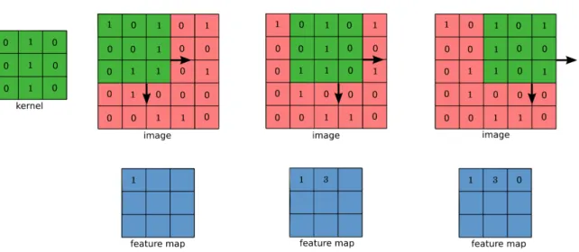
Convolutional Neural Network

Another popular deep learning algorithm is a CNN (LeCun et al., 1990). CNNs are structured slightly differently to MLPs. They often consist of a number of convolu-tional and pooling/subsampling layers followed by fully connected layers (Figure 2.8). Whilst the neurons of the MLP are connected to all neurons in the adjacent layers, the neurons in the convolutional layers of the CNN are only locally connected, and they share weights with other neurons. This can be interpreted as the weights acting

Figure 2.7– An example of a stacked DAE. The input layer is corrupted in some way (e.g. by masking out some of the units), and the network must reconstruct the clean input in the output l