Wavelets and sparse methods for image reconstruction and classification in neuroimaging

(1)

Wavelets and Sparse Methods for Image

Reconstruction and Classification in

Neuroimaging

Michal Piotr Romaniuk

A dissertation submitted in partial fulfilment of the requirements

for the degree of Doctor of Philosphy of Imperial College London

Department of Computing, Imperial College London

(2)

(3)

Declaration of originality

I declare that the work presented in this dissertation is my own, unless specifically acknowledged.

Michal Piotr Romaniuk

(4)

(5)

Copyright declaration

The copyright of this thesis rests with the author and is made available under a Creative Commons Attribution Non-Commercial No Derivatives licence. Research-ers are free to copy, distribute or transmit the thesis on the condition that they attribute it, that they do not use it for commercial purposes and that they do not alter, transform or build upon it. For any reuse or redistribution, researchers must make clear to others the licence terms of this work

(6)

(7)

Abstract

This dissertation contributes to neuroimaging literature in the fields of compressed sensing magnetic resonance imaging (CS-MRI) and image-based detection of Alzheimer’s disease (AD). It consists of three main contributions, based on wavelets and sparse methods.

The first contribution is a method for wavelet packet basis optimisation for sparse approximation and compressed sensing reconstruction of magnetic resonance (MR) images of the brain. The proposed method is based on the basis search algorithm developed by Coifman and Wickerhauser, with a cost function designed specifically for compressed sensing. It is tested on MR images available from the Alzheimer’s Disease Neuroimaging Initiative (ADNI).

The second contribution consists of evaluating and comparing several sparse classification methods in an application to detection of AD based on positron emission tomography (PET) images of the brain. This comparison includes univariate feature selection, feature clustering and classifiers that automatically select a small subset of features due to their mathematical or algorithmic construction. The evaluation is based on PET images available from ADNI.

The third contribution is proposing an extension of wavelet-based scattering networks (originally proposed by Mallat and Bruna) to three-dimensional tomographic images. The proposed extension is evaluated as a feature representation in an application to detection of AD based on MR images available from ADNI.

There are several possible extensions of the work presented in this dissertation. The wavelet packet basis search method proposed in the first contribution can be improved to take into account the coherence between the sparse approximation basis and the sensing basis. The evaluation presented in the second contribution can be extended with additional algorithms to make it more comprehensive. The three-dimensional scattering networks that are the core part of the third contribution can be combined with other machine learning methods, such as manifold learning or deep convolutional neural networks.

As a whole, the methods proposed in this dissertation contribute to the work towards efficient screening for Alzheimer’s disease, by making MRI scans of the brain faster and helping to automate image analysis for AD detection.

(8)

(9)

Acknowledgements

First and foremost, I would like to thank my supervisor Prof. Daniel Rueckert for his support and patience throughout my PhD studies. I would also like to thank my second supervisor Prof. Jo Hajnal for many useful and interesting discussions. I would like to thank Dr Katherine Gray and Dr Robin Wolz for providing processed ADNI data that was used throughout this thesis.

I would like to acknowledge Dr Anil Rao and Dr Kanwal Bhatia for many useful discussions.

I owe very special thanks to Prof. Marek Sergot and Dr Amani El-Kholy. Their dedication and understanding was essential to making the completion of this disser-tation possible.

I would like to acknowledge EPSRC for funding my research and ADNI for providing data that was used throughout this dissertation.

Last but definitely not least, I am grateful to my friends and especially my fam-ily without whose support getting through my PhD studies would not have been possible.

(10)

(11)

Introduction

Imaging technology has had a remarkable impact on medical research and clinical practice in recent decades. Modern imaging tools, such as ultrasonography, magnetic resonance imaging (MRI), computed tomography (CT) and positron emission tomo-graphy (PET) provide the means to produce detailed maps of the internal structure and function of living organisms. This wealth of information allows researchers and practitioners to diagnose diseases more accurately and monitor their progression in unprecedented detail while avoiding many invasive tests.

The development of medical imaging has also prompted interest of computer vision researchers in designing algorithms that derive qualitative and quantitative met-rics from medical images. Within the medical image analysis community, research-ers have proposed numerous algorithms to solve problems such as image registra-tion (estimating spatial correspondence between two or more images), segmentaregistra-tion (partitioning an image into anatomical or functional regions) and computer-aided diagnosis. These tools automate tedious manual tasks, making it easier for medical research to be done efficiently and on a large scale.

In its first part, this introductory chapter covers the basic principles of the medical imaging technologies that were used to acquire the images used in this dissertation: magnetic resonance imaging (MRI) and positron emisson tomography (PET). The second part of this chapter covers some basic background on Alzheimer’s disease, which is important because much of this dissertation is concerned with applying ma-chine learning algorithms to detection of Alzheimer’s disease. Finally, this chapter also enumerates the contributions to the literature made by this dissertation and presents an outline of the remainder of it.

(16)

16 1. INTRODUCTION

1.1. Medical imaging modalities

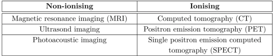
Imaging techniques can be categorised into modalities according to the physical process used to produce the images. Modern imaging modalities can produce three-dimensional tomographic images mapping specific physical properties of tissues across space and each modality has its own specific advantages and disadvantages. Perhaps the most important characteristic describing a modality is whether it uses ionising radiation or not. This is important because ionising radiation poses a health risk. Table 1.1.1 lists several tomographic medical imaging modalities of ionising and non-ionising types.

The remainder of this section presents in some detail the physics of two imaging modalities that were used to acquire the images studied in this dissertation: mag-netic resonance imaging and positron emission tomography.

Table 1.1.1: Selected tomographic medical imaging modalities.

Non-ionising Ionising

Magnetic resonance imaging (MRI) Computed tomography (CT) Ultrasond imaging Positron emission tomography (PET) Photoacoustic imaging Single positron emission computed

tomography (SPECT)

1.1.1. Magnetic resonance imaging. Although quantum mechanical in nature, the physics behind magnetic resonance imaging can be explained in a simplified way using classical principles [109]. The following introduction is based on[179].

MRI relies on a phenomenon called nuclear magnetic resonance. Atomic nuclei with an odd number of protons or neutrons have a property called spin, which can be thought of as associating a tiny magnet with each nucleus. MRI typically focuses on the1_{H (hydrogen-1) nucleus which appears in water and organic molecules.}

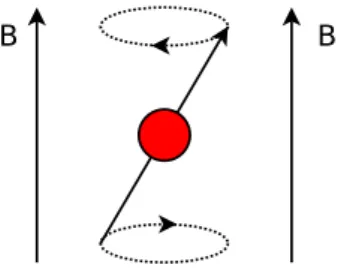
In the presence of an external magnetic field the spins precess about the axis of this field in analogy to the motion of a gyroscope. The direction of alignment is either

(17)

1.1. MEDICAL IMAGING MODALITIES 17

parallel or antiparallel to the direction of field lines, with a small net surplus of spins aligned in parallel, due to the lower energy of this state.

Figure 1.1.1: Precession of a spin can be viewed as similar to the motion of a spinning top.

The frequency of precession is proportional to the strength of the applied magnetic field, according to the Larmor equation:

Ê0 =“B0

whereÊ0is the precession frequency (Larmor frequency),“ is the gyromagnetic ratio

and B0 is the magnetic field. The gyromagnetic ratio of 1H is 42.58 MHz/T, so at

magnetic field strengths generated by main magnets of MR scanners (typically 1.5T or 3T, or in some cases 7T) its Larmor frequency is in the radio frequency (RF) range.

If the nuclei are excited with an RF pulse tuned to the Larmor frequency, the precessive motion of their spins tips away from the direction of the magnetic field. The energy absorbed from the pulse is then re-emitted in the form of radio waves as the spins return to their low-energy state where they are aligned with the field. These radio waves are picked up by a receiver coil and recorded for further processing. The process follows an exponential decay curve and is characterised by a time constant referred to as T1. The variation ofT1 between different types of tissue can be used

as a source of image contrast.

The RF pulse not only causes the spins to tip away from the external magnetic field lines, but also synchronises the phases of their precessive motion [179]. However,

(18)

18 1. INTRODUCTION

this synchrony gradually decays as the individual rates of precession are affected by the electromagnetic interactions between the spins. As a result, the signal at the receiver coil also decays. This process follows an exponential decay curve too, with the time constant T2 associated with it. The differences in T2 between tissues can

be used as an alternative image contrast mechanism.

Spatial encoding in MRI is achieved with additional magnetic field gradients super-imposed on the field generated by the main magnet. These additional gradients are generated with gradient coils installed inside the scanner (shown in figure 1.1.2). Three types of spatial encoding techniques are used to produce three-dimensional images: slice encoding, frequency encoding and phase encoding.

x

y z

Figure 1.1.2: Gradient coils and the MRI coordinate system (radiological conven-tion). The patient is surrounded by three sets of coils (simplified in this diagram)

designed to generate magnetic fields in three directions: x, y and z (red, green and

blue, respectively). The ends of the scanner bore are marked with light blue dashed circles.

Slice encoding is achieved by applying a field gradient during the RF excitation

pulse. This gradient causes Larmor frequency to vary spatially with field strength, so it is possible to excite a thin slice of the sample by shaping the excitation pulse to contain a narrow range of frequencies.

(19)

Spatial encoding in the plane of the slice is achieved by the means of frequency encoding and phase encoding.

Frequency encoding consists of applying a field gradient (orthogonal to the slice

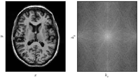
selection gradient) during slice readout, resulting in a proportional variation of Lar-mor frequency across the slice. This means that different temporal frequencies in the signal emitted by the sample represent different locations in space. The signal amplitudes at different temporal frequencies can be recovered from the MR signal with the Fourier transform, giving a one-dimensional distribution of signal in the imaged sample. In other words, the temporal MR signal corresponds to the image in the spatial frequency space (k-space).

Phase encoding relies on applying an additional magnetic field gradient (orthogonal

to both the slice selection gradient and frequency encoding gradient) between fre-quency encoding gradients. The effect of this gradient is to introduce an additional phase shift in the gyration of the spins across the slice, hence the name phase en-coding. This is equivalent to starting a frequency encoding readout along the phase encoding direction ky but interrupting it mid-way through k-space at some kÕ

y, so that now an ordinary frequency encoding readout along kx will capture a part of k-space with ky = kÕy. By repeating the process with different kyÕ, a complete two-dimensional representation of k-space is acquired and this signal is then processed with a two-dimensional Fourier transform to give the spatial image of the slice. Sweeping throughk-space via frequency encoding and phase encoding requires chan-ging the magnetic field within the scanner, which is done by switching currents in the gradient coils. Stronger gradients with rapid switching can in principle give faster scans but also cause problems with peripheral nerve stimulation [54, 122]. This limits the rate at which slices can be acquired, making it difficult to obtain multi-slice images when the patient is moving, e.g. in cardiac imaging or fetal imaging [31, 144].

(20)

20 1. INTRODUCTION

Figure 1.1.3: A brain MRI image (left) and itsk-space representation (right). The T1 and T2 properties change from tissue to tissue, allowing different tissues

to be distinguished. In addition, MRI can be adapted for imaging of diffusion of water molecules (which contain protons) by diffusion weighted imaging (DWI) [14]. Diffusion tensor imaging (DTI) [160] is a related MRI technique that measures the diffusion of water in specific directions. Since water tends to diffuse along the fibers, DTI can be used for tracing neural fibers in the brain [16]. MRI can also be adapted for blood oxygenation dependent (BOLD) contrast, which enables detection of blood flow, which in turn allows for functional imaging [178].

MRI has several advantages as a medical imaging modality. It is non-ionising, which makes it safer than ionising modalities such as CT (which relies on X-rays) and PET (which relies on radioactive tracers). It produces high-resolution images and it offers many useful contrast mechanisms.

The main disadvanage of MRI is the high cost of the scanner and its supporting infrastructure. Additionally, there are dangers associated with imaging patients with metallic implants, which can be subject to large forces and cause damage in the presence of strong magnetic fields, or heat up due to absorbing RF energy.

(21)

MRI scans are used in clinical and scientific applications to study nearly all systems in the human body and they stand out particularly in neuroimaging. With clear contrast between grey matter and white matter, structural T1 scans can be used to study diseases affecting brain structure, including neurodegenerative disease such as Alzheimer’s disease (AD). Diffusion imaging can be used to study the structural connections within the brain and functional MRI can map the brain’s response to sensory stimuli and its functional connectivity.

1.1.2. Positron emission tomography. Positron emission tomography relies on radioactive decay of positron-emitting atomic nuclei to produce images that rep-resent the spatial distribution of these nuclei. When one of these nuclei decays, the emitted positron travels a short distance through the surrounding tissue, losing kin-etic energy due to Coulomb scattering [109]. Once it slows down, it annihilates with an electron, which produces two gamma ray photons emitted in opposite directions [109].

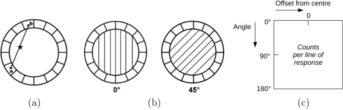
A PET scanner detects gamma ray photons with a ring of gamma ray detectors placed around the patient. The detector ring is equipped with electronics that register events where two detectors receive a gamma ray photon at the same time. When such event occurs, it likely means that the simultaneous detection is due to a positron decaying somewhere on the straight line between those two detectors (called the line of response). These events are counted and their number for each line is recorded. The data is then formatted as a matrix called a sinogram: each row corresponds to a different angle and each column to a different offset from the centre. An image is reconstructed from the sinogram with the filtered back-projection or maximum likelihood expectation maximisation (MLEM) [109].

In order to image a patient with PET, positron-emitting radionuclei are embedded in molecules involved in the biological processes under study and then introduced into the patient’s body. For example, 18_{F-fluorodeoxyglucose (FDG) is commonly}

(22)

22 1. INTRODUCTION

26 Chapter 1. Introduction

of an event determines a path across the detector, known as the line of response, along which the two photons were emitted, as shown in Figure1.5 (a). Parallel lines of response are grouped together to form projections for every possible orientation of the ring, as illustrated in Figure

1.5 (b). The number of events recorded along each line of response in a single projection forms one row of a data matrix called a sinogram. The complete sinogram therefore contains information recorded from all projections in a single ring, as shown in Figure1.5 (c).

(a) Line of response (b) Ring orientations (c) Sinogram

Figure 1.5: Stages of PET image acquisition, showing (a) an annihilation event and the cor-responding line of response, (b) the grouping of parallel lines of response to form projections, and (c) the construction of a sinogram.

Photon attenuation in tissue

At energies around 511 keV, the dominant interaction of photons with tissue is by Compton scattering from outer-shell electrons. This results in both a loss of energy and deflection from the original path. Data must be corrected for errors occuring due to this attenuation, as well as other effects, before an image can be reconstructed. The probability that a photon undergoes no interactions as it travels through tissue along a line l is known as its survival probability. The survival probabilities of the pair of photons produced as shown in Figure

1.5 (a)are independent. The combined probability that neither photon interacts may therefore be expressed as

PC = exp b

a

µ(x)dx

Offset from centre Angle 0 180° 90° 0° Counts per line of response (a) (b) (c)

Figure 1.1.4: PET image acquisition. Left to right: (a) line of response due to positron-electron annihilation, (b) parallel lines of response corresponding to the same angle, and (c) sinogram constructed by grouping detection counts by angle and line

of response. Images (a) and (b) from [109], used with permission; image (c) based on

[109], with changes.

used in neuroimaging as an indicator of cerebral metabolic rate of glucose (CMRgl) [109].

The main advantage of PET as a functional imaging technique is that a radiotracer can be designed to target a specific biochemical process by including a positron-emitting isotope in a molecule involved in that process or a chemically similar mo-lecule. In particular, FDG targets glucose metabolism, which makes it useful in the study of diseases which involve either increased or reduced glucose metabolism. The disadvantages of PET include potential harm due to ionising radiation, low signal to noise ratio (SNR) and high cost.

PET can be used scientifically to study a variety of biochemical processes in the body, depending on the specific radiotracer used. In neuroimaging FDG-PET is used for imaging of Alzheimer’s disease patients because reduced metabolism in specific brain regions was found to be an indicator of AD [155, 195]. Another type of PET scan useful in AD studies uses Pittsburgh compund B (PiB) as radiotracer, which binds to amyloid plaques associated with AD [109].

(23)

1.2. ALZHEIMER’S DISEASE 23

1.2. Alzheimer’s disease

Alzheimer’s disease (AD) is the most common type of dementia, accounting for an estimated 60% to 80% of cases [10]. Its distinctive characteristic is the presence of amyloid beta (Ab) plaques outside neurons and protein tau tangles inside neurons

[10]. The loss of neural cells results in shrinkage of the brain [10].

AD may begin up to 20 years before symptoms appear and progress slowly without causing any effect noticeable to the patient or other people [10]. First symptoms to be noticed often include short-term memory problems and at this stage a person may be diagnosed with mild cognitive impairment (MCI) [10]. Patients diagnosed with MCI have an increased risk of developing AD and other types of dementia, although some of them remain stable or even improve [10]. Probable Alzheimer’s disease is often diagnosed when further decline in memory and cognitive function starts to impair a person’s daily life. In addition to impaired memory, AD symptoms include apathy and depression, problems with language, confusion with time and place, and behavioural changes [10]. Patients with advanced AD lose their ability to communicate, fail to recognise family members and become completely reliant on others for the simplest daily activities and eventually bedbound [10]. A definite diagnosis of AD requires examination of brain tissue samples [109].

1.2.1. Neuroimaging in Alzheimer’s disease. Neuroimaging is used extens-ively in the scientific study of AD. The most established modalities for this applica-tion include structural MRI, FDG-PET and fibrillar AbPET. In addition, functional

MRI, DTI, and several other techniques were also used to learn more about the dis-ease [216].

Structural MRI is used to study the brain atrophy observed in AD. The hippocampus and entorhinal cortex of AD patients have reduced volume, gray matter and cortical thickness [216]. Many other cerebral regions are also affected [216]. Meanwhile, sulcal and ventricular volumes are larger in AD [216]. The presence of these changes

(24)

24 1. INTRODUCTION

in asymptomatic subjects and higher rate of their progression indicate an increased risk of developing MCI or AD [216].

FDG-PET is used to map CMRgl across the brain. In AD patients CMRgl is reduced in the posterior cingulate, precuneus and parietotemporal regions [155]. More advanced AD also affects CMRgl in the frontal cortex and the rest of the brain [216]. These changes correlate with disease severity and they also have predictive value [216].

AD patients Normal controls

MR I (T1 ) FD G -P E T

Figure 1.2.1: MR T1-weighted (top) and FDG-PET (bottom) images of AD patients (left panel) and cognitive normal controls (right panel).

Fibrillar AbPET is used to study the deposition of amyloid beta plaques in the brain

[216]. This technique was used to confirm Ab deposits in the brains of affected

patients, particularly in the precuneus, posterior cingulate, parietotemporal and frontal regions [216]. In addition, these studies suggested that fibrillar Ab PET

levels are already near saturation in patients with MCI [216]. Fibrillar Ab PET is

expected to play an important role in evaluation of potential AD treatments that aim to clear Ab deposits or prevent their accumulation [216]. These tests will also

(25)

1.3. CONTRIBUTIONS 25

The Alzheimer’s disease neuroimaging intiative (ADNI) is a longitudinal observa-tional study of a large group of Alzheimer’s disease patients, MCI patients and a matched group of cognitively normal controls [197]. ADNI is a multisite collab-oration with subjects receiving regular, standardised MR and (for some of them) PET scans, in addition to neuropsychologic, genetic and cerebrospinal fluid testing [197, 135, 137]. Anonymised data can be accessed by researchers as a unified database. The goals of ADNI are to develop standardised imaging protocols for AD and MCI studies, collect structural and metabolic imaging data, validate imaging biomarkers against standard clinical and cognitive measures, compare biomarkers with respect to their utility for AD and MCI diagnosis and tracking of effects due to treatment, and to create a generally accessible data repository [197]. ADNI data was used in a large number of scientific papers and the success of the initiative prompted its extension to ADNI-GO and ADNI2 stages [262].

1.3. Contributions

The contributions of this dissertation include applications of wavelets, sparse rep-resentations and machine learning to the problems of compressed sensing MRI re-construction and image-based classification of Alzheimer’s disease.

• The contribution to compressed sensing consists of adapting the wavelet packet best basis search algorithm [55, 56] for application to MR image re-construction from undersampled data. An optimised basis is learned from a set of brain MR images from the ADNI database. This basis is shown to rep-resent both training images and unseen brain images in a more sparse way than standard wavelets. The optimised basis is also compared to standard wavelets in reconstruction of brain MR images from simulated compressed sensing data. In the context of the rest of this dissertation, compressed sensing can be used to accelerate MRI scans for detection of AD, allowing

(26)

26 1. INTRODUCTION

for more patients to be examined. This work was presented at the 2012 MICCAI Workshop on Sparsity Techniques in Medical Imaging [217]. • The first contribution to image-based classification consists of comparing

several dimensionality reduction methods for AD detection based on FDG-PET data. Several feature selection and clustering algorithms are tested with a range of different classification algorithms to evaluate the poten-tial benefits of feature selection in FDG-PET based AD detection. The algorithms are compared with respect to their classification performance as well as the distribution of selected features throughout the brain.

• The second contribution to image-based AD detection consists of extending the invariant scattering convolution network architecture proposed recently by Bruna and Mallat [27] to three-dimensional tomographic images and applying this image representation to the problem of AD detection based on MR images. The problems due to the very large dimensionality of 3D scattering data are addressed by applying the fast Johnson-Lindenstrauss transform introduced recently by Ailon and Liberty [5] as a form of data compression. The classifiers are learned and applied in the compressed domain, enabling efficient learning and classification in a situation where practical challenges would appear with learning from full-dimensional data. As a whole, the work presented in this dissertation is aimed at making AD screening and prediction more accessible, by improving the efficiency of brain MRI scanning and developing tools for computer-assisted diagnosis of AD and detection of its early signs.

1.4. Thesis outline

The remainder of this dissertation is organised as described in the following.

Chapters 2 and 3 introduce the relevant background. Chapter 2 covers wavelet representations in signal processing as well as sparse representations and compressed

(27)

1.4. THESIS OUTLINE 27

sensing. Chapter 3 presents an overview of the machine learning techniques that are used in subsequent chapters.

Compressed sensing MRI with optimised wavelet packet representations is discussed in chapter 4. The wavelet packet basis search algorithm [55, 56] is adapted for finding an optimally sparse wavelet packet basis for a set of images. This algorithm is then evaluated by fitting a wavelet packet basis to a set of brain MR images and measuring the sparsity of representations of other brain MR images in this basis. The adapted basis is also compared with wavelets in an application to MRI reconstruction from compressed sensing k-space data.

Sparse algorithms for image-based classification of Alzheimer’s disease are discussed in chapter 5. Feature selection steps are added to several classification algorithms and these composite classifiers are evaluated on FDG-PET brain images of Alzheimer’s disease patients and cognitive normal (CN) subjects. Those trained classifiers are also evaluated on the task of predicting whether an MCI patient will progress to AD or remain stable.

In chapter 6 scattering networks introduced by Bruna and Mallat [27] are extended to three-dimensional tomographic images. In addition, a fast Johnson-Lindenstrauss transform introduced by Ailon and Liberty [5] is proposed as a method to reduce the dimensionality of scattering network output to make application of machine learning more practical. These algorithms are then evaluated on MRI data from ADNI by classifying between AD patients and controls and in addition making predictions of whether MCI patients will progress to AD or remain stable.

Chapter 7 presents the outlook for the topics discussed in previous chapters, with a discussion of potential extensions of the work presented.

(28)

(29)

CHAPTER 2

Wavelets, sparsity and compressed sensing

In signal and image processing it is common to represent signals as sums of simple elements often referred to as atomic signals or simply atoms. Those representations make it possible to extract features of signals that may not be immediately appar-ent, or ones that appear salient to a human observer but difficult to distinguish automatically with an algorithm. Perhaps the most widely known example of this is the Fourier representation which models signals as sums of sinusoids or complex exponentials [187].

2.1. Wavelets

The sinusoids used as atomic signals in Fourier analysis have the benefit of distin-guishing frequencies with high resolution but they are unable to localise the features of a signal in time (or space for spatial signals such as images). This has prompted the development of alternative representations which can localise signals in time (or space) at the expense of loss of some frequency resolution.

Wavelet transforms describe signals as sums of scaled and shifted versions of an atomic waveform known as the “mother wavelet”. Large-scale atoms can provide a rough approximation of a signal. Meanwhile, compactly supported atoms add detail near discontinuities, such as edges in images. Large values of wavelet coefficients in the small scales appear near edges [187] while uniform regions have small coefficients at those scales, which enables efficient image compression.

(30)

30 2. WAVELETS, SPARSITY AND COMPRESSED SENSING

Some basic concepts from wavelet theory are presented in the following. Since the subject of wavelets is very broad, this discussion is limited to the topics that are relevant to the algorithms discussed in further chapters.

2.1.1. Continuous wavelets in one dimension. A continuous wavelet ana-lysis can be defined by choosing a mother wavelet, i.e. a function Â(t) such that

´Œ

≠Œ|Â(t)|

2

dt = 1 and ´Œ

≠ŒÂ(t)dt = 0 [187] where the second condition means that the wavelet averages out to zero over its support. The “daughter wavelets” at scale s œ R+ and translation u œ R are then derived from the mother wavelet as follows [187]. Âu,s(t) = Ô1 sÂ 3_t_≠_u s 4

A function f(t)œL2(R) is transformed into its wavelet representation FÂ(u, s) as

follows [187].

FÂ(u, s) = Èf,Âu,sÍ=

ˆ Œ

≠Œ

f(t)Âú_u,s(t)dt

The following theorem shows that the signalf(t)can be reconstructed fromFÂ(u, s)

(Âˆ(Ê)denotes the Fourier transform of Â(t)).

Theorem 1. (Calderon, Grossman and Morlet. This version quoted from [187])

“LetÂ _œL2(R) be a real function such that

(31)

2.1. WAVELETS 31

In other words, under a mild condition (equation 2.1.1) on the wavelet function, the continuous wavelet transform is invertible (with the inverse given by equation 2.1.2), and preserves signal energy up to a constant factor (as shown by equation 2.1.3).

The constantCÂ ensures that reconstruction with equation 2.1.2 returns the original

f(t) rather than its scaled version.

Note that the condition in equation 2.1.1 (called the wavelet admissibility condition [187]) implies that it is necessary thatÂˆ(0) = 0. In other words, this explains why the average of the wavelet over its support must be zero [187].

The theory discussed so far explains how to transform continuous functions of time (or space) into wavelet representations that are continuous in time (or space) and scale. These results are important from a theoretical perspective but in computa-tional applications the function to be transformed and the wavelet representation must both be discrete. The simplest way of addressing this problem is to sample the signal and its wavelet representation. The sampling rate of the signal is chosen so as to ensure that no information is lost due to aliasing. The sampling rate of the wavelet transform is often chosen so that the scale is on a logarithmic grid and the time intervals are matched to each scale individually. More specifically, [105] (2.1.4) s= 2d, u=n2d, nœZ, dœZ

whered controls scale and n controls translation.

The Gabor wavelet is a commonly used wavelet defined as a continuous function. It consitsts of a complex exponential modulated by a Gaussian window [187]:

ÂG(t) = 1

(‡2ﬁ)1/4 exp (iÊ0t) exp

A ≠ t 2 2‡2 B .

This function is not a wavelet in the strict sense because it does not average out to zero. However, this problem can be addressed by a simple adjustment, giving the

(32)

Morlet wavelet [27]:

Â(t) =–(exp (iÊ0t)≠—) exp

A ≠ t

2

2‡2

B

where— is chosen so that´

Â(u)du= 0[27]. The Morlet wavelet is shown in figure 2.1.1.

Figure 2.1.1: Morlet wavelet (real part in solid blue, imaginary part in dashed red).

2.1.2. Discrete wavelets in one dimension. An alternative way to define wavelet transforms is to start with multirate filter banks and scaling functions. The structure of a filter bank implementing the discrete wavelet transform (DWT) and the corresponding reconstruction filter bank are shown in figure 2.1.2. The filters h0[n], h1[n], g0[n] and g1[n] are chosen to ensure perfect reconstruction

(y[n] =x[n]).

Figure 2.1.2: Discrete wavelet decomposition (left) and reconstruction (right).

The perfect reconstruction condition leaves some freedom to the designer of the filter banks, allowing other objectives to be met. For example, compact support of the

(33)

2.1. WAVELETS 33

filters (i.e. finite length of their impulse responses) is a convenient property because it allows a very efficient implementation with Mallat’s multiresolution analysis al-gorithm [188]. The filters can be designed to be orthogonal, so that the wavelet transform is also orthognal [187].

Daubechies wavelets [66] are a commonly used family of orthogonal, compactly supported wavelets. The Daubechies family consists of a wavelet for each integer number of vanishing moments of the filter g[n], with a minimal support length for that number of vanishing moments, allowing these wavelets to represent polynomials very efficiently [187].

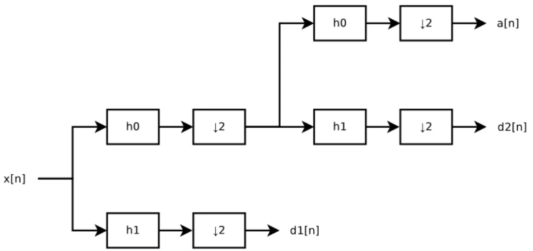
A multi-level discrete wavelet decomposition is obtained by iterating the filter bank in figure 2.1.2 on the low-pass branch. For example, the filter tree in figure 2.1.3

decomposes its input into two detail bands and one approximation band. The corres-ponding reconstruction filter tree is shown in2.1.4. Mallat’s multiresolution analysis algorithm uses these filter trees to implement a fast wavelet transform [188].

Figure 2.1.3: Multi-level discrete wavelet decomposition.

Filter banks used for a discrete wavelet transform can be used to derive a continuous wavelet and the associated scaling function (the basis function associated with the approximation band) using an iterative refinement algorithm [66, 30]. The db4

(34)

Figure 2.1.4: Multi-level discrete wavelet reconstruction.

Figure 2.1.5: Thedb4scaling function, wavelet and decomposition filters h0[n]and h1[n].

Discrete wavelet transforms can easily be expressed as matrix multiplication of a transform matrix and a signal vector [30]. The transform matrix is formed from the basis vectors of the wavelet representation as rows, and both single-level and multi-level transforms can be represented in this way. In computational applications the direct implementation of filter banks is much faster but the matrix representation is helpful in the analysis of theoretical aspects of the discrete wavelet transform.

(35)

2.1. WAVELETS 35

Unless the signals are of infinite duration, both continuous and discrete formulations of wavelets have to handle boundary conditions. Some extension (padding) of the signal has to be assumed at the start and end of the signal. Periodic padding (i.e. concatenating a copy of the signal before its start and after its end) is elegant from a mathematical point of view because the associated transform matrix is circulant and with orthogonal filter banks it is also orthogonal. The disadvantage of this approach is that it often introduces a discontinuity at the point of concatenation. An alternative apprach is symmetric padding, where a reversed version of the signal is concatenated at both of its ends. This avoids the discontinuity but orthogonality is lost.

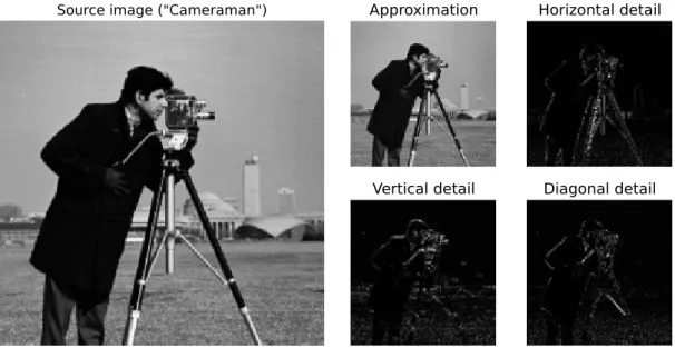
2.1.3. Image processing with wavelets. Discrete wavelet transforms for im-ages are computed by applying the filters h0[n] and h1[n] to all rows of an image

individually and then to the columns of the resulting representation. After down-sampling, this gives four frequency bands: approximation, horizontal detail, vertical detail and diagonal detail. Alternatively, the frequency bands can be computed by pre-computing a two-dimensional kernel for each frequency band and convolving it with the image, followed by downsampling.

An example of a single-level two-dimensional wavelet decomposition is shown in figure 2.1.6. A multi-level decomposition for images is obtained by iterating the single level decomposition on the approximation band.

This definition of a wavelet transform for images is easily extended to three-dimensional tomographic images by applying a third pair of filters along thez-direction. A multi-level decomposition is then derived analogously by iterating the filter bank on the approximation band.

An alternative way of applying wavelets to images is to define a set of directional filters with different orientations. The filters have a band-pass profile along their longitudinal axis and low-pass profile along the transverse axis (or axes in case of

(36)

Figure 2.1.6: Single-level 2D wavelet decomposition. The source image (left) is the standard “Cameraman” test image. To the right, the approximation and directional detail bands. Note that the intensities of the images on the right were individually

rescaled to cover the grayscale colour range,i.e. they are not directly comparable in

terms of coefficient size.

3D), which makes this method useful for detecting edges (in 2D) or surfaces (in 3D). There are several transforms of this type, including wedgelets [76], bandelets [161], curvelets [40] and shearlets [154, 115].

2.2. Sparse representations

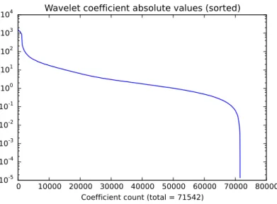
Since wavelet atoms are localised and separate data into different scales, they can approximate images in a sparse way. The low-pass bands are sufficient to recon-struct smooth regions in an image with good accuracy so the detail bands in the corresponding regions are close to zero and their ommision would have little effect on the quality of the image. This can be seene.g. in figure 2.1.6, where only a small proportion of coefficients in the detail bands are significantly far from zero. Figure 2.2.1 shows the decay of coefficients in the wavelet representation of the “Camer-man” image with three levels of decomposition. When the image is reconstructed from approximately 10% of its largest wavelet coefficients, the result (figure 2.2.2) is very close to the original.

(37)

2.2. SPARSE REPRESENTATIONS 37

Figure 2.2.1: Decay of weavelet coefficients. The plot shows absolute values of

wave-let coefficients for the “Cameraman” image, with three levels of wavelet decomposition.

Note logarithmic vertical axis.

Figure 2.2.2: Left: sparse wavelet image reconstruction of the “Cameraman” image

(shown in figure 2.1.6) from approximately 10% of its wavelet coefficients with largest

absolute values. Right: error map of this reconstruction.

Sparsity in the strict sense can be defined as follows.

Definition 2. (Tropp, [251]) s-sparse vector

A vector x is said to be s-sparse if ÎxÎ0 Æ s where Î.Î0 is a function that returns

(38)

2.2.1. Optimising for sparsity. Orthogonal transforms provide unique rep-resentations for signals, so optimal approximations for different sparsity-accuracy trade-offs are easily obtained by setting the smallest coefficients to zero until the rquired level of sparsity is reached. However, non-orthogonal dictionaries require more advanced algorithms to find optimal sparse approximations.

Consider the representation equationx=D“ wherexœRm is the vector represent-ing the (discrete) signal, D œ Rm◊n is the matrix representing the dictionary, with atoms as columns, and “ œ Rn is the vector of representation coefficients. With an overcomplete dictionary this system is underdetermined, with no unique solution. This means that there is some freedom in choosing a representation. This problem can be written as [251]

(2.2.1) min

“œRnÎ“Î0 s.t. x=D“

where Î“Î0 is the ¸0 pseudonorm, i.e. the nomber of non-zero components of the

vector“.

It turns out that the problem in equation 2.2.1 is very difficult to solve compu-tationally. Some algorithms such as matching pursuit (MP) [189] and orthogonal matching pursuit (OMP) [202] can find solutions that are typically suboptimal (but these algorithms are fast). Alternatively, under some conditions ([78, 77]; also see the discussion on compressed sensing below) it is possible to solve an ¸1 version of

the problem in equation 2.2.1,i.e.

(2.2.2) min

(39)

2.2. SPARSE REPRESENTATIONS 39

and with large probability get a solution that is also optimal for 2.2.1. The problem 2.2.2 is known in signal processing as basis pursuit [45]. It is a linear optimisation problem that has been studied extensively by mathematical optimisation researchers and a number of efficient algorithms are known that can be used to find a solution, as discussed by Tropp and Wright [251].

The discussion so far focused on the problem of sparse representation,i.e. finding a combination of atoms that represents a signal exactly. However, in reality this might not be the right problem to solve because the model with all signals composed of a small number of atoms each is an idealised one. A more realistic approach is to allow a trade-offbetween sparsity and aproximation error, which gives the following optimisation problem.

(2.2.3) min

“œRn 1

2ÎD“≠xÎ22+⁄Î“Î1

This problem is known as basis pursuit denoising (BPDN) [45]. It can also be written in two alternative forms, as follows.

min “œRnÎ“Î1 s.t. 1 2ÎD“≠xÎ22 Æ‘2 (2.2.4) min “œRn 1 2ÎD“≠xÎ22 s.t. Î“Î1 Æ· (2.2.5)

Both of those two problems can be transformed into the form in equation 2.2.3 using the method of Lagrangian multipliers. The BPDN problem can be solved computationally with several types of algorithms, which are discussed in detail by Tropp and Wright [251].

In statistics the problem in equation 2.2.5 is also referred to as least absolute shrink-age selection operator (LASSO) [246].

(40)

2.2.2. Adpative sparse dictionaries. Sparse representations can also be con-structed adaptively, by matching the dictionary of atomic signals to a particu-lar image or set of images. This problem is referred to as dictionary learning [198, 152, 3, 141, 88, 269, 29, 165, 250, 213]. It can be formulated math-ematically as (2.2.6) min DœRm◊n_,_“_œ_Rn 3₁ 2Îx≠D“Î22+⁄Î“Î1 4

which is essentially the same problem as the one in formula 2.2.3, except that the minimisation is overD in addition to “, making it much more difficult to solve. Dictionary learning literature was reviewed by Tosic and Frossard [250]. The K-SVD algorithm [3] is worth mentioning in particular. It alternates between sparsely representing an image in a set of atoms and optimising the atoms, with efficient implementations for both of these steps.

Dictionary learning algorithms are usually applied to small image patches [198, 3, 86, 141, 185, 186, 87, 220, 165], rather than whole images which is the case with wavelets. Therefore, sparsity in dictionary learning is accomplished in the sense of individual patches being sparse in the learned dictionary of patch-size atoms. Olshausen and Field [198] found that the atoms in a dictionary optimised (with a cost function slightly different from the one in equation 2.2.6 and a different optimisation algorithm) for patches of natural images resembled directional wavelets. The sparsity of wavelet transforms can be improved with adaptive wavelet packet representations [55, 56]. Wavelet packets are an extension of discrete wavelets where filter banks are iterated on the high-pass branches in addition to low-pass branches. An adaptive wavelet packet representation is then built by choosing the point in each branch where the iteration should stop. In contrast to the dictionary learning algorithms discussed above, a wavelet packet basis is normally optimised for a whole image or set of images instead of image patches. Wavelet packets are discussed in detail in chapter 4.

(41)

2.3. COMPRESSED SENSING 41

2.3. Compressed sensing

Compressed sensing (or compressive sensing) [36, 38, 42, 82], abbreviated as CS, is a mathematical signal processing technique that can be used to reconstruct sparse signals from a reduced number of linear measurements. A compressed sensing system can be modeled with the equation

(2.3.1) y=A“

where yœRm is the vector of measurements, A_œ _Rm◊n is the sensing matrix and “ œ Rn is the sparse vector that is being measured. We can think of _“ as being in the “sparse representation space” andy as being in the “sensing space”.

This model can easily accommodate the case where we are trying to reconstruct a data vector x in a “human readable space” which is not itself sparse but can be represented sparsely in another basis,i.e. when x=D“ as discussed in section 2.2. In this case we have

y= D“

where is the “physical” sensing matrix that transforms an object from its natural representation (e.g. pixels or voxels) to compressive measurements. This reduces to 2.3.1 when A = D, i.e. when we consider the system as a whole to be taking direct linear measurements of the sparse representation.

The structure of the matrix depends on the particular sensing system under con-sideration. For example, in magnetic resonance imaging is a matrix constructed from a subset of rows of the Fourier transform matrix.

(42)

2.3.1. Restricted isometries. Intuitively, to enable reconstruction of sparse signals, it is necessary for the matrix A to transform different sparse vectors “ into different measurement vectors y. Otherwise, if there were sparse vectors “1 and “2

such that y = A“1 = A“2, it would be impossible to distinguish “1 and “2 based

only on their measurement vectors with any method. More formally, we define

the restricted isometry property, which is characterised by the restricted isometry

constant of a matrix.

Definition 3. (Originally Candes and Tao [38], this version from [34]) Restricted

isometry constant

For each integers, the restricted isometry constant ”s of a matrixA is the smallest number such that

(1≠”s)Î“Î22 Æ ÎA“Î22 Æ(1 +”s)Î“Î22

holds for all s-sparse vectors “.

Essentially, this definition formalises the requirement that the transformation A

only distorts the square of the¸2 norm of any s-sparse vector to a degree limited by

”s.

If we consider twos-sparse vectors“1 and “2, the¸0 pseudo-norm of their difference

is at most 2s. Therefore, the restricted isometry constant ”2s places a limit on the degree to which the pairwise distances betweens-sparse vectors can be distorted by the transformationA [39].

Intuitively, it makes sense to have a matrix A with ”2s that is as close to 0 as pos-sible, since this results in Euclidean distances between sparse vectors only becoming distorted to a small degree by the transformation defined by A. In order for A to encode s-sparse vectors unambiguously, it is necessary that ”2s < 1, which ensures

(43)

2.3. COMPRESSED SENSING 43

that there are no2s-sparse vectors in the null space of A and thus that reconstruc-tion by ¸0 minimisation has a unique solution [39]. Matrices with good restricted

isometry constants can be generated using random matrix constructions (with high probability) [15, 34] or deterministically [74].

2.3.2. Noiseless compressed sensing recovery. Returning to the model in equation 2.3.1, the signal “ usually is not sparse in the strict sense but a sparse approximation can be constructed with a small number s of its components with the largest magnitude. Let us denote this approximation as“s. As already discussed in section 2.2, such approximations can be very accurate even whensis small relative to the dimension of “ if the right representation is chosen (see figure 2.2.1 for the wavelet example). The aim of compressed sensing recovery is to reconstruct“s from

y.

Compressed sensing reconstruction essentially consists of using a sparse coding al-gorithm to find the sparsest vector“ı that is consistent with the measurements seen

in y. In particular, when ¸1 minimisation is used as the reconstruction algorithm,

the following theorem states the requirements for exact reconstruction of“s.

Theorem 4. Noiseless recovery [34]

If y=A“ and the matrix A has the restricted isometry constant ”2s <

Ô 2≠1 and “ı is the solution to min ˜ “œRnÎ“˜Î1 s.t. A˜“ =y then Î“ı_≠“_Î₁ _ÆC0Î“≠“sÎ1 and

(44)

||“ı ≠“||2 ÆC0||“≠Ô“s||1

s

for some constantC0. In particular, if “ is s-sparse, the recovery is exact.

This theorem means essentially that if the sensing matrix transformation does not distort the pairwise distances between s-sparse vectors too much, then ¸1

minim-isation recovers an s-sparse vector exactly. In addition, if the vector “ is only approximately sparse, then the reconstruction error is bounded by the error of the s-sparse approximation multiplied by a constant. This is important because it es-tablishes that compressed sensing with¸1 reconstruction is still effective when signal

representations are only approximately sparse [39].

2.3.3. Noisy compressed sensing recovery. In reality the model 2.3.1 with approximate sparsity is still somewhat idealised in the sense that it does not include noise in the system. The model of a noisy compressed sensing system is

y=A“+z wherez is the noise term.

The following theorem then puts a bound on reconstruction error for reconstruction with ¸1 minimisation.

Theorem 5. Noisy recovery [34]

If y=A“ +z and the matrix A has the restricted isometry constant ”2s <

Ô₂ ≠1

and ÎzÎ2 ÆÁ and “ı is the solution to

min

˜

(45)

2.4. APPLICATIONS TO NEUROIMAGING 45

then

(2.3.2) Î“ı_≠“_Î₂ _ÆC0Î“≠Ô“sÎ1

s +C1Á

for some constantsC0 and C1. In particular, if “ is s-sparse, the recovery is exact.

The constants C0 and C1 are quite reasonable: for example, when ”2s = 0.2, the error in 2.3.2 is bounded by 4.2Î“≠_Ô“sÎ1

s + 8.5Á [34].

Theorem 5 establishes that reconstruction error of ¸1 recovery scales linearly with

both sensor noise and approximation error of the sparse signal model. Therefore, compressed sensing with ¸1 recovery is robust, which is important for practical

ap-plications of this theory.

2.4. Applications to neuroimaging

Wavelets and sparse methods have found many applications in neuroimaging. Sev-eral authors applied wavelet analysis to the problem of statistical testing of activ-ation maps in fMRI analysis [23, 222, 71, 196, 92, 28, 258, 146, 201]. These methods are an alternative to conventional statistical parametric mapping (SPM) [103]. Wavelets are useful in fMRI analysis because of their denoising property: piece-wise smooth signals can be approximated closely by a relatively small number of large coefficients while noise is distributed evenly, so wavelet shrinkage tends to improve signal quality [81, 80]. Since wavelet analysis eliminates the requirement of image smoothing with Gaussian filters to reduce noise, these wavelet methods can map brain activity with higher resolution [196].

Voxel-based morphometry (VBM) [9], which allows SPM to be applied to struc-tural brain images, was extended with wavelets by Canales-Rodriguez et al. [33].

(46)

Classification of Alzheimer’s disease using structural MRI and the dual-tree com-plex wavelet transform was proposed by Hackmack et al. [117]. Lao et al. [156] proposed a method for morphological classification of brain images that uses the discrete wavelet transform to enable efficient reduction of data dimensionality. Dictionary learning was applied in the neuroimaging context to fMRI analysis [163, 255, 85], hippocampus segmentation [248], lesion segmentation [263] and brain atlas construction [229].

Neuroimaging is also an important application of compressed sensing. MRI was used as an example application in early work on CS by Candes et al. [36] and a complete CS-MRI system was soon built by Lustig et al. [183, 181], using the discrete wavelet transform and image instensity variation for sparsifying structural MR images. Extensive literature on compressed sensing MRI is available, with a recent review by Hollingsworth available in [132]. Compressed sensing was also combined with dictionary learning for MR imaging [211, 236]. Chapter 4 starts with a more detailed discussion of compressed sensing MRI techniques that represent images with adaptive sparse dictionaries.

2.5. Conclusions

This chapter introduced some basic concepts in wavelets, sparsity and compressed sensing. The discrete wavelet transform is a prerequisite for wavelet packets which chapter 4 is focused on. Morlet wavelets are used in chapter 6 as a building block of scattering networks. Sparsity is important in chapter 5 where classification al-gorithms with¸1 regularisation are evaluated alongside other methods. Next chapter

introduces basic concepts in machine learning, including several classification al-gorithms.

(47)

CHAPTER 3

Machine learning

Machine learning (ML) is the study of algorithms that adapt to data, with par-ticular emphasis on algorithms that detect nontrivial patterns or make predictions about future or missing data. The field of machine learning is closely related to computational statistics and those two fields intersect and inspire each other. Machine learning problems can be divided into supervised learning and unsupervised learning. Supervised learning is concerned with problems where the reference values of the target variables (“ground truth”) are available for the instances in the train-ing set. Supervised learntrain-ing models learn by adjusttrain-ing their internal variables so that their outputs predict target variables based on input variables (predictors). Su-pervised learning can be categorised into regression (predicting a continuous-valued target variable) and classification (predicting a discrete-valued label).

Unsupervised learning is concerned with problems where reference values of the outputs are not available but patterns are still sarched for. Clustering, where one seeks to group data into clusters of similar samples, is an example of an unsupervised learning problem.

3.1. Classification

Classification is a type of supervised learning where the goal is to predict a discrete-valued label. For example, one may be interested in predicting based on an MR image if a patient would be diagnosed as healthy, suffering from MCI or from AD (three possible labels). This section is intended to provide the background on the

(48)

48 3. MACHINE LEARNING

three classification algorithms that are used later in this dissertation: logistic re-gression, support vector machines and random forests.

3.1.1. Logistic regression. Logistic regression relies on the logit transforma-tion to build a model that predicts class probabilities for each feature vector x. A fitted logistic regression model can be used for classification by selecting the label that has the highest predicted probability for a given vector of predictors.

For the case of two classes, the predicted class probabilities are as follows [123].

Pr (Y = 1_|X =x;—) = exp 1 —Tx2 1 + exp (—Tx) Pr (Y = 0|X =x;—) = 1 1 + exp (—Tx)

where(X, Y) _œRp+1_◊_{0_,1_} is a random variable that represents data points and their labels. We use(xi, yi), iœ[1, . . . , n]to denote a specific sample. It is assumed that the feature vector x has a “1” prefixed to allow for an intercept in the model (i.e. x=5 1 x1 · · · xp

6

) and — is a vector with the same dimension as x. The semicolon is used to separate variables from model parameters.

Given a set of training data (xi, yi), i œ [1, . . . , n], a logistic regression model is fitted by maximising the log-likelihood of the data in the following way (derivation based on [123]).

The log-likelihood of the data given the model is ¸(—) =

n

ÿ

i=1

log Pr (Y =yi_|X=xi;—) which can be written as

¸(—) = n

ÿ

i=1

(49)

3.1. CLASSIFICATION 49

which ensures that whenyi = 1 we take log Pr (Y = 1_|X=xi;—), and when yi = 0 we take log Pr (Y = 0|X =xi;—). After substituting the logistic regression probab-ility model and simplifying, this becomes

¸(—) = n ÿ i=1 Ë yi—Txi≠log 1 1 + exp1—Txi 22È . The derivative with respect to — is

ˆ¸(—) ˆ— = n ÿ i=1 xi S Uyi_≠ exp 1 —Tx i 2 1 + exp (—Tx i) T V.

This expression can be used to find the maximum with gradient descent or alternat-ively the Hessian can also be derived to enable solution with the Newton-Raphson method [123].

3.1.2. Overfitting and regularisation. If the number of features available for building a machine learning model such as logistic regression is large enough then it is possible to fit the data in a near-perfect way. However, the data available for training in most cases only represents a limited number of samples at a limited number of points in the feature space. In addition, data often contains noise, such as imperfect measurements or incorrect labels. The source of the the data may also be probabilistic in nature, with labels depending on features in a way which is to some degree random. These issues can lead to a problem called overfitting, where the model fits the training data very well but fails to generalise to new data. The problem of overfitting can be alleviated by including a regularisation term in the cost function. Most commonly, regularisation is based on ¸1 or ¸2 norm of the

weight vector — (excluding the intercept —0).

The ¸1 version is fitted by solving the following optimisation problem [123].

max — Q a n ÿ i=1 Ë yi—Txi≠log 1 1 + exp1—Txi 22È ≠⁄ n ÿ j=2 |—_j| R b

(50)

50 3. MACHINE LEARNING

The ¸2 version is similar, with the following optimisation problem.

max — Q a n ÿ i=1 Ë yi—Txi≠log 1 1 + exp1—Tx i 22È ≠⁄ n ÿ j=2 —_j2 R b

These are maximisation problems, so the norm has to be included with negative sign so that smaller values of the norm are preferred.

Regularisation biases the solution towards smaller weights, reducing model variance. If the weight of the regularisation term is adjusted well then the reduction in variance outweighs the bias introduced and generalisation performance improves relative to the unregularised model.

The regularisation term treats the coefficients associated with all predictors (ex-cept for the inter(ex-cept) equally, so it is common to normalise the predictors be-fore applying regularised logistic regression [123]. Algorithms for solving regular-ised logistic regression problems computationally were proposed by several authors [283, 284, 145, 102, 273, 247].

If there are more than two classes, the logistic regression model can be extended to accommodate that requirement, although this results in more mathematical com-plexity. Alternatively, it is possible to use a two-class version in a one-vs-rest frame-work. In this case a classifier is built for each class that can distinguish that class from all other classes combined in one set. The class label prediction is then assigned as the class with the highest probability as computed by its own vs-rest classifier. Another alternative framework for multi-class classification is one-vs-one, where a classifier is trained to distinguish between each pair of classes and the class label prediction is the class with the most pairwise tests resolved in its favour.

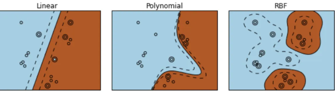
3.1.3. Support vector machines. The idea of support vector machines (SVM) [254] is to find a hyperplane that separates data points so that the two classes are on opposite sides of the hyperplane and there is a maximum possible margin between

(51)

3.1. CLASSIFICATION 51

the hyperplane and any of the points. The derivation of the SVM optimisation problem below is adapted from [123].

Figure 3.1.1: Classification problem with samples from two groups (marked with

different colours). The separating hyperplane is marked with a solid line. The dashed

lines bound the maximum margin. The samples at the edges of the margin (marked with larger circles) are the support vectors. (Image generated with Scikit-learn ex-ample code.)

A hyperplane is defined by the equation

xT_—₊_—

0 = 0

where x œ Rp is a point on the hyperplane, _— _œ _Rp is the normal vector of the hyperplane and—0 œRis a scalar. The signed distance of an arbitrary pointxfrom

this plane is [123] d= 1 Î—_Î₂ 1 xT_—₊_— 0 2

The sign of d is of particular interest because it indicates on which side of the hyperplane the point x lies. The problem of finding a separating hyperplane that maximises the margin can then be written as

(3.1.1) max —,—0 M s.t. zi 1 Î—Î2 1 xT i —+—0 2 ØM, i= 1, . . . , n

where M is the margin and zi _œ _{_≠1,1_} are the respective labels for the training instancesxi,≠1for one class and1for the other. As argued in [123], “since for any