Abstract — In this paper we present a new algorithm based on the Bee Colony Optimization (BCO) meta-heuristic for the Multidimensional Knapsack Problem (MKP), the goal of which is to find a subset of objects that maximizes a given objective function while satisfying some resource constraints. We show that our new algorithm obtains better results than Ant Colony Optimization algorithms and on most instances it reaches best known solutions. Especially we propose an efficient algorithm to produce randomly new solutions.
Index Terms — Bee Colony Optimization, Multidimensional Knapsack Problem.
I. INTRODUCTION
Multidimensional Knapsack Problem is a NP-hard problem which has many practical applications, such as processor allocation in distributed systems, cargo loading, or capital budgeting. The goal of the MKP is to find a subset of objects that maximizes the total profit while satisfying some resource constraints. More formally, a MKP is stated as follows:
maximize
∑
n
j
=
1
c
j.x
jsubject to
n
ij jb
i1
j
=
a
.x
≤
∑
∀i∈1..m
x
j∈
{
0
,
1
}
∀
j
∈
1
..
n
, where aij is the consumption of resource i for object j, bi is
the available quantity of resource i, cj is the profit associated
with object j, and xj is the decision variable associated with
object j and is set to 1 (resp. 0) if j is selected (resp. not selected).
This problem was solved by using Ant Colony Optimization [1]-[3], genetic algorithm [4], and Tabu search [5]. In this paper we describe a new algorithm for solving MKPs. This algorithm is based on BCO, a stochastic meta-heuristic that has been applied to solve combinatorial optimization problems such as job shop scheduling problems, multi-agent systems, or ride-matching problem in the transportation domain. For more details about BCO algorithm, the reader referred to [6], [7]. Here we only produce basic ideas and model of this algorithm in Section 2. The mappings of multidimensional knapsack to honey bees forager deployment is then described in Section 3, including describing two extra characteristics of bee colony and two corresponding definitions in subsections 3.1, 3.2, and
Manuscript received January 7, 2008.
Papova Nhina Nhicolaievna - Moscow State University, Russia. Le Van Thanh - MSU, Russia ([email protected]).
concretizing the BCO algorithm for MKP in subsections 3.2, 3.3, 3.4. In Section 4 we give efficient parameters in experiment. Subsequently, comparative study on the performance of the BCO approaches on the benchmark problems in Section 5.
II. GENERAL MODEL OF BCO ALGORITHM
There are two major characteristics of the bee colony in searching for food sources: waggle dance and forage (or nectar exploration). First scout bees search for food randomly from one flower patch to another. They evaluate the different patches according to the quality of the food and the amount of energy usage. And then they return to hive, communicate through a waggle dance which contains information about the direction of the flower patch (angle between the sun and patch), the distance from the hive (duration of the dance) and the quality rating (frequency of the dance). Using the information received from the waggle dance, bees go to the patch to gather food. According to the fitness, patches can be visited by more bees or may be abandoned.
Relying to these features, a model of BCO algorithm was proposed as figure 1. The algorithm requires a number of parameters to be set, namely: number of scout bees (nBee), number of sites selected for neighborhood search (out of nBee visited sites) (nSite
≤
nBee), the initial size of each patch (ngh) (a patch is a region in the search space that includes the visited site and its neighborhood), number of bees recruited for the selected sites (nep) (these bees will try to find better solutions in the correlative patch of selected site), and the stopping criterion.Algorithm_1:
1. Initialize population with nBee random solutions. 2. Evaluate fitness of the population.
3. While (stopping criterion not met)
3.1. Select nSite sites for neighborhood search. 3.2. Determine the patch size (ngh).
3.3. Recruit nep bees for selected sites and evaluate fitnesses.
3.4. Select the representative bees from each patch. 3.5. Assign remaining bees to search randomly and
evaluate their fitnesses.
Figure 1. Pseudo code of the BCO algorithm
This model and detailed models of BCO in this paper don’t present clearly the role of waggle dance, but reader could see an example of using waggle dance in [8].
Bee Colony Algorithm for
the Multidimensional Knapsack Problem
III. APPLYING BCO TO MULTIDIMENSIONAL KNAPSACK
This section details algorithms to perform Multidimensional Knapsack inspired by the behavior of honey bee colony. The fitness of a solution is value of sum
∑
n
j
=
1
c
j.x
j. Let nIteration be number of iterations ofstep 3 until the present and maxIteration be the bound of nIteration then stopping criterion of algorithm_1 is equivalent to condition nIteration >= maxIteration. First we put forward an extra characteristic of bee colony, which is real interesting and efficient for increasing rate of search the best solution in a huge space.
A. Lived time of Food Source
In the nature, each food source is harvested by bee colony for a certain time, which depends on the abundance of food source and amount of bees visited it. Therefore, we define the lived time of a food source x, denoted by livedT(x), to be the number of iterations of step 3 since food source was found indispensable to harvest out of food. It means each selected site x will be searched for better solution in maximum livedT(x) iterations. After this period, candidate solution x will be abandoned even if it is the best solution.
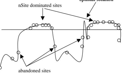
Figure 2 helps us imagine the usefulness of lived time: after a certain number of iterations of step 3, dominated solutions converge to local maxima, and search for better solution around these solutions is almost meaningless. The fitness of these solutions is big enough to prevent new random solutions from being selected to nSite dominated sites. So that nSite selected sites for local search is almost unchanged between two consecutive iterations of step 3. The only way to find the optimal solution is wait a luckiness of search randomly in step 3.5.
optimal solution nSite dominated sites
[image:2.595.51.292.484.630.2]abandoned sites
Figure 2. A state of the BCO algorithm
B. Distribution Function and Algorithm for Production Randomly New Solutions
Unlike most of other heuristics for MKP, BCO produces a certain amount of random solutions in each circle, besides initial solutions in step 2. Therefore a good algorithm for production new solution affects considerably to convergent rate of the BCO algorithm. We will discuss some points to build a good enough algorithm.
Let vector x = (x0, x1, …, xn) be a solution of MKP and pj be
probability of xj = 1 (j
∈
___
,
1
n
). Then this probability depends on cj, aij (i∈
___
,
1
m
) (the bigger cj and the smaller aij, thebigger pj). So that formula to define pj like below:
pj = f * (cj)
α
/ (∑
i
a
ij)β
, where f – some function (1)It’s probably that cj is much bigger than aij. In this case the
role of aij in (1) is not considerable (i.e. pj depends on cj more
than on
∑
i
a
ij ). But in fact values of cj and aij are unrelated.It means we need a formula of pj, in which the role of cj and aij
is equivalent to each other. Let maxC be maximum value of cj
and maxS be maximum of
∑
i
(a
ij /∑
t
a
it ) then
pj = f * (cj / maxC)
α
/ {(∑
i
(a
ij /∑
t
a
it )) / maxS}β
(2)In formula (2) interrelation between cj and aij depends on
values of
α
andβ
. However in some cases formula (2) unsuccessfully shows the roles of aij. For example, if existsh-th constraint bh ~
∑
t
a
ht then this constraint is satisfiedeven if most of xt equal 1, i.e. probability of xj = 1 depends
little on ahj. Let ahj be much bigger than other aht, pj in (2)
considerably depends on ahj. Therefore we have next
formula:
pj = f*(cj/maxC)
α
/{(∑
i
(a
ij / (bi*∑
t
a
it )))/maxS’}β
(3), where maxS’ be maximum of
∑
i
(a
ij / (bi*∑
t
a
it )).If probability function only has a simple formula like (3) where f doesn’t depend on time, then the BCO algorithm rapidly converges to some local maxima. For this reason we propose a new definition – distribution function, denoted by df. This function describes another characteristic of bee colony in nature that patches of food source, where were visited more times in past, will be reduced visitation because of decrease of food’s quality. Value of function is measured by number of visitations by bees. For MKP, we concretize df as follows:
df(j) = number of visited solutions x in steps 2, 3.4 and 3.5, j-th element of which is 1 (xj = 1).
Function df(j) depends on time and pj depends on df(j). We
pj(
α
,β
,γ
) = fj * (maxDF / df(j))γ
* (cj / maxC)α
/{(
∑
i
(a
ij / (bi*∑
t
a
it ))) / maxS’}β
(4), where maxDF is current maximum of df(t) (t
∈
___
,
1
n
). The following algorithm for production new solutions bases on formula (3). But first we say roulette wheel selection again, because we will use it to make random for the BCO algorithm.Suppose we have n objects, each object has a particular probability of selection. Our task is taking one from them. Roulette wheel selection consists of following steps:
1. Generate a random number in [0,
∑
probabilit
y
].2. For i from 1 to n:
If sum of probabilities from 0 to i reaches or exceeds upper random number then i is selected object and stop algorithm.
Denote rws(g, O) to be function realizes roulette wheel selection for object set O on probability function g, this function returns selected element. Algorithm for production new solutions as follows:
Algorithm_2:
1. For (j
∈
___
,
1
n
):1.1 Generate a random number in {0, 1, 2}. If this number equals 0 then fj = probability0,
otherwise fj = probability1.
1.2 Assign 0 to xj.
2. Initialize object set S, including n elements from 1 to n. 3. While (|S| > 0): S isn’t empty
3.1 Assign 1 to xt, where t = rws(p(
α
,β
,γ
), S).3.2 S = S/{t
∪
break-set}, where break-set = {j∈
S/{t} |∃
i: aij +∑
=
1
x
a
r
ir > bi}.
Most of previous algorithms for initializing population assign 0 or 1 each bit of x according to a random number being 0 or 1. In algorithm_2 we have a change, a random number is also generated but this value only uses to determine probability of each bit of x to be 1. If this number is 0 then corresponding bit has less possibility of getting 1 (set0) than in case this number isn’t 0 (set1). So that values probability0 and probability1 are added, satisfy probability0 < probability1. In 1.1 we choose set {0, 1, 2} to make number of bits of set1 more than one of set0. It’s only a tricky but in experiment this choice gives satisfactory results, so that we produce it here in order to readers consult.
C. Definition of Patch Size
Let set Jx = (j0, j1, …) be set of indexes, which correspond
with bits 1 of x, i.e.
Jx
j
x
j∈
= 1 andj
Jx
x
j∉
= 0. Then a vectorx* = (x*0, x*1, …, x*n) belongs to the k-neighboring region
of x (k
≤
|Jx|), which means x* is produced from x byfollowing algorithm:
Algorithm_3:
1. Choose a set Jk of k elements from Jx, assign 0 to each
element of it and evaluate pj(
α
’,β
’,γ
’) with fj =probability0’, j
∈
Jk .2. For each bit j’
∉
Jx evaluate pj’(α
’,β
’,γ
’) with fj’ =probability1’.
3. Let S = Jk
∪
[J /{Jx}].4. While (|S| > 0):
4.1 Assign 1 to xt, where t = rws(p(
α
’,β
’,γ
’), S).4.2 S = S/{t
∪
break-set}, where break-set = {j∈
S/{t} |∃
i: aij +∑
=
1
x
a
r
ir > bi}.
, where probability0’ and probability1’ have meaning similar to probability0 and.probability1. Note that in step 1, if j-th
bit of x has dominated corresponding cj and non-dominated
sum
∑
i
(a
ij / (bi*∑
t
a
it )) then probability of it to be 1 isbig. Hence, we choose set Jk as follows: 1. Let S = Jx. Jk = {}.
2. While (|S| < k):
2.1 t = rws(1/p(
α
’’,β
’’,γ
’’) with f = 1, S). Add t to Jk.2.2 S = S/{t}.
Above, we described almost all details of the BCO algorithm. Following, we discuss last part of this algorithm – neighborhood search.
D. Neighborhood Search
Neighborhood or local search moves from an initial solution by a sequence of neighborhood changes, which improve each time the value of the objective function until a local optimum is found. The connectivity property pertaining to local search states that starting with any feasible solution, there exists some sequence of moves that will reach an optimal solution. Neighborhood structures play a very important role in local search as the time complexity of a search depends on the size of the neighborhood and the computational cost of the moves.
For our algorithm, each solution is a local optimum, i.e. if we change state of any bit of it then either some constraint is broken (from 0 to 1) or fitness of solution decrease (from 1 to 0). So that for neighborhood search of x we execute by algorithm_4:
Algorithm_4:
1. bf = fitness of x. 2. For (k
∈
_______
,
2
ngh
): For (i∈
_______
2.1. Choose a random solution, which belongs to the k-neighboring region of x.
2.2. Evaluate its fitness. If this value greater than bf then update bf.
3. If bf > fitness of x then replace x with solution, corresponding to bf, lived time of x to be restarted (= 0).
In algorithm_4 we change some (
≥
2) bits 1 of solution to 0, and then complete bits 0 (change state to 1) to set Jx. Itmeans that we changed from one local optimum to other optimum, and hoped its fitness will be better than the first’s. But using the same values of ngh and nep for each solution of nSite selected sites isn’t sensible because it intensifies executing time of algorithm. Therefore we split nSite sites to 2 classes : best class and better class. Best class includes nBest bees, which have best fitness out of nBee bees, and better class includes (nSite – nBest) bees, which have next best fitness. Each class has particular values nep and livedT (nepb, livedTb for best ones and nep, livedT for better one). And fully worked-out model of the BCO algorithm consists of following steps:
Algorithm_5:
1. Initialize population with nBee random solutions with old = 0. nIteration = 0.
2. Evaluate fitness of the population. 3. While (nIteration < maxIteration)
3.1. Select nSite and nBest sites for neighborhood search.
3.2. Determine the patch size (ngh).
3.3. Recruit nepb (and nep) bees for selected sites with old < livedTb (and livedT) to search around these sites by algorithm_4.
3.4. Select the representative bees from each patch (if the representative bee is root bee than old++ otherwise old= 0).
3.5. Assign remaining bees to search randomly with old = 0 and evaluate their fitnesses.
Figure 3. Pseudo code of the BCO algorithm for MKP
IV. PARAMETERS SETTING
When solving a combinatorial optimization problem with a heuristic approach such as evolutionary computation, ACO or BCO, one usually has to find a compromise between two dual goals. On one hand, one has to intensify the search around the most “promising” areas that are usually close to the best solutions found so far. On the other hand, one has to diversify the search and favor exploration in order to discover new, and hopefully more successful, areas of the search space. The behavior of bees with respect to this intensification/diversification duality can be influenced by modifying parameter values, including maxIteration, nBee, nSite, nBest, nep, nepb, ngh, livedT,
α
,β
,γ
,α
’,β
’,γ
’,α
’’,β
’’,γ
’’, probability0, probability1, probability0’, probability1’.It’s too many parameters to survey, thus we fix some parameters after some times of test runs:
maxInteration ~ 500
nBee = 600, nSite = 100, nBest = 10, ngh = 5, livedTb = 30, livedT = 20,
α
=β
= 1,γ
= 2,α
’=β
’=γ
’= 1,α
’’= 2,β
’’= 1,γ
’’= 0,probability0 = 0.2, probability1 = 0.8, probability0’ = 0.1, probability1’ = 0.9.
Then that we used a set of MKP instances with 100 objects and 5 resource constraints to find sensible values of parameters nep and nepb. Results that in about 200 seconds, and nIteration ~ 400 the algorithm finds almost best known solutions with pair parameters (nep ~ 40, nepb ~ 120). Increasing nepb, value nIteration to find best solutions is reduced (time to find it increases considerably), but increasing nep has no more effective. Otherwise both decreasing nep and nepb reduce qualities of solutions, and the algorithm rapidly converge to local maxima.
For all experiments reported below, we have set nep to 8% of n.m and nepb to 24% of n.m.
V. EXPERIMENTS AND RESULTS
Data set, rely on which to compare to other approaches, is benchmarks of MKP from OR-Library. We compare the results of the BCO algorithm with the two ACO algorithms of Leguizamon and Michalewicz [2] and Alaya, Solnon and Ghedira [3], and the genetic algorithm of Chu and Beasly [4].
Table_1 is results on 100 x 5 instances. For each instance, the table reports the best solutions found by Chu and Beasley as reported in [4] (C. & B.), the best and average solutions found by Alaya, Solnon and Ghedira as reported in [3] (A., S. & G.), and the best and average solutions found by Leguizamon and Michalewicz as reported in [2] (L. & M.), the best, average solutions, probability of successfully and average number of iterations to find best solution of the BCO algorithm_5 over 50 runs. Table_2 is results on 100 x 10 instances. And Table_3 is results on new benchmarks of MKP in http://hces.bus.olemiss.edu (over 10 runs).
In Table_3, we see that the results are not good enough, because sizes of data set are large. We guess a cooperative BCO be conformable to this data set. The BCO algorithm only runs well with medium (~ 100 x 10) search space.
VI. CONCLUSION
Table_1:
№ C. & B. A., S. & G. L. & M. BCO
Best Best Avg Best Avg Best Avg % N
01 24381 24381 24342 24381 24331 23381 23377.8 70% 223 02 24274 24274 24247 24274 24245 24274 24274.0 100% 84 03 23551 23551 23529 23551 23527 24551 24545.3 56% 237 04 23534 23534 23462 23527 23463 23534 23519.5 32% 278 05 23991 23991 23946 23991 23949 23991 23985.0 76% 196 06 24613 24613 24587 24613 24563 24613 24613.0 100% 101 07 25591 25591 25512 25591 25504 25591 25591.0 100% 79 08 23410 23410 23371 23361 23204 23410 23410.0 100% 99 09 24216 24216 24172 24173 23762 24216 24216.0 100% 142 10 24411 24411 24356 24411 24326 24411 24409.2 94% 144 11 42757 42757 42704 42757 42756.0 98% 183 12 42545 42510 42456 42545 42519.6 28% 323 13 41968 41967 41934 41968 41955.8 6% 272 14 45090 45071 45056 45090 45079.3 44% 227 15 42218 42218 42194 42218 42199.0 22% 315 16 42927 42927 42911 42927 42927.0 100% 121 17 42009 42009 41977 42009 42009.0 100% 117 18 45020 45010 44971 45020 45015.8 80% 223 19 43441 43441 43356 43441 43400.4 44% 274 20 44554 44554 44506 44554 44539.4 74% 279 21 59822 59822 59821 59822 59822.0 100% 31 22 62081 62081 62010 62081 62081.0 100% 109 23 59802 59802 59759 59802 59801.2 96% 164 24 60479 60479 60428 60479 60479.0 100% 112 25 61091 61091 61072 61091 61091.0 100% 82 26 58959 58959 58945 58959 58959.0 100% 87 27 61538 61538 61514 61538 61538.0 100% 153 28 61520 61520 61492 61520 61520.0 100% 131 29 59453 59453 59436 59453 59453.0 100% 73 30 59965 59965 59958 59965 59965.0 100% 149
Table_2:
№ C. & B. A., S. & G. L. & M. BCO
Best Best Avg Best Avg Best Avg % N
01 23064 23064 23016 23057 22996 23064 23060.9 52% 279 02 22801 22801 22714 22801 22672 22801 22791.1 74% 212 03 22131 22131 22034 22131 21980 22131 22129.0 96% 116 04 22772 22717 22634 22772 22631 22772 22758.9 32% 234 05 22751 22654 22547 22654 22578 22751 22722.9 50% 250 06 22777 22716 22602 22652 22565 22777 22727.3 20% 322 07 21875 21875 21777 21875 21758 21875 21874.6 98% 132 08 22635 22551 22453 22551 22519 22635 22621.6 84% 201 09 22511 22511 22351 22418 22292 22511 22492.3 72% 160 10 22702 22702 22591 22702 22588 22702 22702.0 100% 107 11 41395 41395 41329 41395 41385.3 42% 281 12 42344 42344 42214 42344 42302.9 40% 218 13 42401 42401 42300 42401 42372.6 46% 198 14 45624 45624 45461 45624 45576.4 8% 311 15 41884 41884 41739 41884 41862.2 50% 218 16 42995 42995 42909 42995 42995.0 100% 109 17 43559 43553 43464 43574 43548.0 6% 320
18 42970 42970 42903 42970 42968.6 96% 153 19 42212 42212 42146 42212 42212.0 100% 92 20 41207 41207 41067 41207 41149.2 10% 332 21 57375 57375 57318 57375 57375.0 100% 28 22 58978 58978 58889 58978 58978.0 100% 103 23 58391 58391 58333 58391 58379.4 60% 171 24 61966 61966 61885 61966 61964.9 98% 124 25 60803 60803 60798 60803 60803.0 100% 24 26 61437 61437 61293 61437 61403.5 52% 223 27 56377 56377 56324 56377 56371.2 76% 176 28 59391 59391 59339 50391 50391.0 100% 40 29 60205 60205 60146 60205 60205.0 100% 72 30 60633 60633 60605 60633 60633.0 100% 28
Table_3:
№ Size n x m Best known solution BCO
Best Avg % N
01 100 x 15 3766 3758 3753 10% 225 02 100 x 25 3958 3951 3947 20% 360 03 150 x 25 5650 5637 5629 20% 342 04 150 x 50 5764 5741 5737 10% 113 05 200 x 25 7557 7531 7529 20% 237 06 200 x 50 7672 7640 7635 20% 134
REFERENCES
[1] S.Fidanova, “Evolutionary algorithm for Multidimensional Knapsack Problem”.
[2] G.Leguizamon and Z.Michalewicz, “A new version of Ant System for Subset Problem”.
[3] I.Alaya, C.Solnon and K.Ghedira, “Ant algorithm for the multidimensional Knapsack Problem”.
[4] P.C.Chu and J.E.Beasley, “A Genetic algorithm for the Multidimentional Knapsack Problem”.
[5] Michel Vasquez and Jin-Kao Hao, “A Hybrid Approach for the 0–1 Multidimensional Knapsack problem”.
[6] D.T.Pham, A.Ghanbarzadeh, “Multi-Objective Optimisation using the Bees algorithm”.
[7] D.T.Pham , A.Ghanbarzadeh, E. Kos, S. Otri, S. Rahim, M. Zaidi, “The Bees algorithm – a novel tool for Complex Optimisation Problems”.