Software Defect Prediction Using Enhanced
Machine Learning Technique
Soumya Joseph1 , G.P.Simi Margaret2
M. Tech Student, Dept. of CSE, Marian Engineering College, Trivandrum, Kerala, India1
Asst. Professor, Dept. of CSE, Marian Engineering College, Trivandrum, Kerala, India 2
ABSTRACT: Software defect prediction plays an important role in maintaining high quality software and reducing the cost of software development. It facilitates project managers to allocate time and resources to defect-prone modules through early defect detection. Software defect prediction is a binary classification problem which classifies modules of software into either of the 2 categories: Defect–prone and not-defect-prone modules. Misclassifying defect-prone modules as not-defect-prone modules leads to a higher misclassification cost than misclassifying not-defect-prone modules as defect-prone ones. The machine learning algorithm used in this paper is a combination of Cost-Sensitive Variance Score (CSVS), Cost-Sensitive Laplace Score (CSLS) and Cost-Sensitive Constraint Score (CSCS). The proposed algorithm is evaluated and shows better performance and low misclassification cost when compared with the 3 algorithms executed separately.
KEYWORDS: Cost-Sensitive learning; feature selection; Software defect prediction
I. INTRODUCTION
Sdp can be defined as a binary classification problem, where software modules are classified as either defect -prone or not-defect--prone modules, using a set of software metrics. the common software metrics include: cyclomatic complexity, halstead complexity, number of lines of code ect. most software defect prediction studies have utilized machine learning techniques. the first step to build a prediction model is to generate instances from software archives such as version control systems, issue tracking systems, e-mail archives, and so on. each instance can represent a system, a software component (or package), a source code file, a class, a function (or method), and/or a code change according to prediction granularity.
After generating instances with metrics and labels, we can apply pre-processing techniques, which are common in machine learning. Pre-processing techniques used in defect prediction studies include Feature selection, Dimension reduction, Classification, Prediction and finally Performance analysis. The flow chart below depicts the entire process of software defect prediction. The historical data, including various software metrics captured from software systems, are divided into two groups: the training data set, and the test data set. These data are pre-processed before being fed into the following feature selection and classification algorithms. In the second stage, cost-sensitive feature selection algorithms are applied to the training data to find the optimal features, and thus the dimension can be reduced. The next step is to train the cost-sensitive classification models based on the training data set with selected features.
With the final set of training instances, we can train a prediction model..The prediction model can predict whether a new instance is defect prone or not-defect-prone.
II. RELATEDWORK
metrics are extracted from software archives such as version control systems and issue tracking systems that manage all development histories. Process metrics quantify many aspects of software development process such as changes of source code, ownership of source code files, developer interactions, etc. Usefulness of process metrics for defect prediction has been proved in many studies.
Most defect prediction studies are conducted based on statistical approach, i.e. machine learning. Prediction models learned by machine learning algorithms can predict either bug-proneness of source code (classification) or the number of defects in source code (regression. Defect prediction models tried to identify defects in system, component/package, or file/class levels. Recent studies showed the possibility to identify defects even in module/method and change levels. Finer granularity can help developers by narrowing the scope of source code review for quality assurance.
Proposing preprocessing techniques for prediction models is also an important research branch in defect prediction studies. Before building a prediction model, we may apply the following techniques: feature selection, normalization, and noise handling. With the preprocessing techniques proposed, prediction performance could be improved in the related studies. Researchers also have proposed approaches for cross-project defect prediction. Most representative studies described above have been conducted and verified under the within-prediction setting, i.e. prediction models were built and tested in the same project. However, it is difficult for new projects, which do not have enough development historical information, to build prediction models. Representative approaches for cross defect prediction are metric compensation Nearest Neighbor (NN) Filter, Transfer Naive Bayes, These approaches adapt a prediction model by selecting similar instances, transforming data values, or developing a new model.
III.ENHANCEDFEATURESELECTION
Feature selection has been widely used in many pattern recognition and machine learning applications for decades. The aim of feature selection is to find the minimally sized feature subset that is necessary and sufficient for a specific task. The proposed algorithm is obtained by adding the 3 novel cost sensitive algorithms cost sensitive variance score, cost sensitive laplacian score and cost sensitive constraint score to formulate a new equation. The features are first extracted on the basis of the 3 algorithms. The features thus obtained are then combined together and given as input to the proposed algorithm to generate a new set of features.
Variance score (VS) is a simple unsupervised evaluation criterion of features. It selects features that have the maximum variance among all samples, with the basic idea that the variance among a feature space reflects the representative power of this feature. As another popular unsupervised feature selection method, Laplacian Score (LS) not only prefers features with larger variances which have more representative power, but also prefers features with stronger locality preserving ability Constraint Score(CS) is a semi-supervised feature selection method, which performs feature selection according to the constraint preserving ability of features It uses must-link and cannot-link pair-wise constraints as supervision information, where features that can best preserve the must-link constraints as well as the cannot-link constraints are assumed to be important.
Existing feature selection methods designed for SDP are cost-blind, i.e., the issue of different costs for different errors is not considered. The proposed algorithm is obtained by adding the 3 novel cost sensitive algorithms cost sensitive variance score, cost sensitive laplacian score and cost sensitive constraint score to formulate a new equation. The features are first extracted on the basis of the 3 algorithms. The features thus obtained are then combined together and given as input to the proposed algorithm to generate a new set of features.[4]
IV.COST-SENSITIVELEARNING
The measure of performance of a machine learning algorithm is based on its accuracy of classifying a data set. In most real-world applications; different misclassifications are usually associated with different costs. [2]Denote class labels as {1…c}. Misclassifying a sample from the ith class as the c th class will cause higher costs than misclassifying a sample of the c th class as other classes. Here, we call the class from the 1st class to the (c-1) th class the in-group class, while the c th class is called the out-group class. Then, we can categorize misclassification costs into three types: 1) the cost of false acceptance, i.e., the cost of misclassifying a sample from the out-group class as being from the in-group class; 2) the cost of false rejection, i.e., the cost of misclassifying a sample from the in-group class as being from the out-group class; and 3) the cost of false identification, i.e., the cost of misclassifying a sample from one in-group class as being from another in-group class. To represent the differing cost of each type of misclassification, a cost matrix given below can be used.[5]
Defect-prone Not-defect-prone Defect -prone C(0,0)=c00 C(0,1)=c01
Not-defect-prone C(1,0)=c10 C(1,1)=c11
Fig 1:Cost Matrix
V. PREDICTION
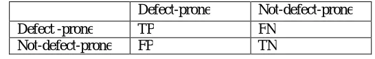
The features extracted using enhanced feature selection are used in the test data and checked if the value falls within the range. The result of prediction can be expressed as a confusion matrix show below.
True positive(TP) : defect prone module predicted as defect prone. False positives(FP) : not-defect-prone module predicted as defect-prone.
True negative(TN) : not-defect-prone module predicted as not-defect-prone module. False negative(FN) : defect prone module predicted as not-defect-prone.
Defect-prone Not-defect-prone Defect -prone TP FN
Not-defect-prone FP TN
Fig 2:Confusion matrix
VI.PERFORMANCEANALYSIS
For better evaluating the performances in the cost-sensitive learning scenarios, the Total-cost of misclassification, which is a general measurement for cost-sensitive learning, is used as one primary evaluation criterion in our experiments. On the other hand, as shown in Fig 2, the classification results can be represented by the confusion matrix with two rows and two columns reporting the number of true positives (TP), false positives (FP), false negatives (FN), and true negatives (TN).
TP
Sensitivity = …….. (1) TP+FN
(TP+TN)
Accuracy = ……… (2)
Where sensitivity measures the proportion of defect-prone modules correctly classified, and accuracy measures the proportion of samples correctly classified among the whole population. In addition to the Total-cost, we also adopt the sensitivity and accuracy of the classification results as evaluation measures.
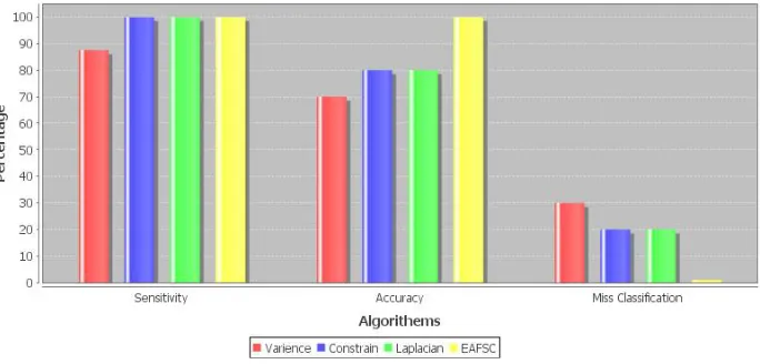
Fig 3: Comparison of different feature selection algorithms
One can observe that the enhanced algorithm have much lower misclassification cost than CSVS,CSLS,CSCS.
It also has better accuracy when compared to the other 3 algorithms. The Sensitivity is also comparable to the other three algorithms.
VII. CONCLUSION
The enhanced algorithm is obtained by adding 3 cost-sensitive algorithms namely Cost-Sensitive Variance Score (CSVS), Cost-Sensitive Laplace Score (CSLS) and Cost-Sensitive Constraint Score (CSCS).From experiments on the dataset collected from NASA, its observed that the enhanced algorithm produces better performance than when the 3 algorithms are executed separately.
REFERENCES
1. Mingxia Liu, LinsongMiao, and Daoqiang Zhang, “Two-Stage Cost-Sensitive Learning for Software Defect Prediction,” IEEE Transactions on reliability, Vol. 63, No. 2, June 2014.
2. P. D. Turney, “Cost-sensitive classification: Empirical evaluation of a hybrid genetic decision tree induction algorithm,” J. Artif. Intell. Res., vol. 2, pp. 369–409,2011.
3. I. Guyon, S. Gunn, M. Nikravesh, and Z. L. , Feature Extraction:Foundations and Applications. Berlin, Germany: Springer-VerlagNew York, Inc., 2006.
4. D. Sun and D. Zhang, “Bagging constraint score for feature selection with pairwise constraints,” Pattern Recogn., vol. 43, pp. 2106–2118,2010. 5. C. Seiffert, T. M. Khoshgoftaar, J. V. Hulse, and A. Napolitano, “A comparative study of data sampling and cost sensitive learning,” in Proc.
IEEE Int. Conf. DataMiningWorkshops,Washington, DC, USA, 2008, pp. 46–52.
6. Z.-H. Zhou and X.-Y. Liu, “On multi-class cost-sensitive learning,” in Proc. 21st National Conf. Artificial Intelligence, 2006,pp.567–572. 7. A. Bernstein, J. Ekanayake, andM. Pinzger, “Improving defect prediction using temporal features and non linear models,” in 9th Int. Workshopon
Principles of Software Evolution, Dubrovnik, Croatia, 2007, pp. 11–18.
8. Y. Bo and L. Xiang, “A study on software reliability prediction based on support vector machines,” in Proc. IEEE Int. Conf. Ind. Eng. Eng.Manag., Singapore, 2007, pp. 1176–1180.
10. S. Kim, Z. T. J. Whitehead, and A. Zeller, “Predicting faults from cached history,” in Proc. 29th Int. Conf. Software Eng., Washington, DC, USA, 2007, pp. 489–498.
11. R. Moser, W. Pedrycz, and G. Succi, “A comparative analysis of the efficiency of change metrics and static code attributes for defect prediction,” in Proc. 30th Int. Conf. Software Eng., Leipzig, Germany, 2008, pp. 181–190.
BIOGRAPHY