R E S E A R C H
Open Access
A novel distributed fusion algorithm for
multi-sensor nonlinear tracking
Jingxian Liu
1, Zulin Wang
1,2†and Mai Xu
1*†Abstract
The covariance intersection (CI), especially with feedback structure, can be easily combined with nonlinear filters to solve the distributed fusion problem of multi-sensor nonlinear tracking. However, this paper proves that the CI algorithm is sub-optimal, thus degrading the fusion accuracy. To avoid such an issue, a novel distributed fusion algorithm, namely Monte Carlo Bayesian (MCB) algorithm, is proposed. First, it builds a distributed fusion architecture based on the Bayesian tracking framework. Then, the Monte Carlo sampling is incorporated into this architecture to form a feasible solution to nonlinear tracking. Finally, the simulation results verify that our MCB algorithm advances the state-of-the-art distributed fusion of nonlinear tracking.
Keywords: Bayesian tracking framework, Monte Carlo sampling, Covariance intersection
1 Introduction
Distributed fusion [1] refers to combining the information of decentralized sensors [2, 3], in which the observation information of each sensor is processed independently. In comparison with centralized fusion, the distributed fusion can significantly save time and storage resources in the fusion center. As for distributed fusion, the conven-tional solution is Bar-Shalom-Campo algorithm [4]. Later, Chang et al. [5] proved that this algorithm is not opti-mal in terms of the root-mean-square-error (RMSE), and they further presented an optimal fusion algorithm. Nev-ertheless, this algorithm can only be used in the scenario of two sensors fusion. Hence, Li et al. [6] proposed a uni-fied fusion architecture, which can be used for two and more sensors. However, all aforementioned algorithms are designed with linear state space models (SSM), which results in the inferior fusion performance of nonlinear tracking.
Recently, some intelligent techniques, such as the adap-tive fuzzy backstepping control technique [7] and the adaptive neural network technique [8] with nonlinear model predictive control, are proposed to advance the application of nonlinear models in multi-sensors or sensor
*Correspondence: [email protected]
†Equal contributors
1School of Electrical and Information Engineering, Beihang University, XueYuan Road No.37, Haidian District, 100191 Beijing, China Full list of author information is available at the end of the article
network control [9]. Hence, the optimal distributed fusion with nonlinear model becomes one of the most important direction of signal processing. To our best knowledge, the most effective algorithms for fusion are based on covari-ance intersection (CI) [10, 11]. These CI-based algorithms can be easily combined with nonlinear filers to form the state-of-the-art solutions to nonlinear problems, such as UKF-SCI [12] and DPF-ICI [13]. The former is more accu-rate because the unscented Kalman filter (UKF) performs better in normally nonlinear tracking, while the latter has an advantage in non-Gaussian scenarios benefitting from the particle filter (PF). However, these CI-based algo-rithms require the computation on additional fractional powers to calculate the fusion results [14], which causes an increment of estimation error. Although many applica-tions utilize a feedback structure1 to improve the fusion
accuracy [15], this paper proves that the sub-optimality caused by the increment of estimation error still exists in CI. To our best knowledge, few algorithms are proposed to overcome this sub-optimality. Hence, the present study is motivated to achieve a fusion algorithm which can out-perform the CI algorithm. In summary, the novelty of this paper is that our algorithm overcomes the sub-optimality problem in covariance intersection (CI) fusion, which has not been addressed in the previous work.
In this paper, a Monte Carlo Bayesian (MCB) algorithm is proposed to overcome the disadvantage of the sub-optimality in CI algorithm, such that the fusion perfor-mance can be improved. Specifically, a distributed fusion architecture is designed based on the Bayesian track-ing framework (BTF). This algorithm utilizes the law of total probability to form the distributed architecture, thus avoiding the increment of estimation error. Furthermore, the Monte Carlo sampling [16] is incorporated into our distributed architecture. This sampling method offers a direct approximate inference of the expectation of the tar-get function with respect to a probability distribution [17]. Benefiting from this sampling method, the intractable problem of nonlinear estimation in BTF is circumvented by means of the approximation algorithm with sampling particles. Finally, based on the approximation, the fusion results are achieved in the form of the mean and variance of estimation at each step. The meanings of notation in the paper are listed in Table 1. The contributions of this work are listed as follows,
• A novel distributed fusion architecture is proposed, which makes full use of the information of different sensors to produce robust fusion estimation.
Table 1Notation list
Notation Meaning of the notation
xk The state at time stepk
Pk The variance of state at time stepk
i Thei-th sensor
I The number of sensors
n Then-th particle
N The number of particles
Xnk Then-th particle of state at time stepk zik The observation of thei-th sensor at time stepk zf1:k The observation set of all sensors from time step 1 tok p(·) The transition distribution of state
q(·) The likelihood of state
hi(·) The observation function of thei-th sensor
Q The variance of observation noise
δ(·) The Dirac delta function
C The normalized constant
F The transition function
nk−1 The transition noise at timek−1
dx,k,dy,k The distances alongxandydirection at time stepk vx,k,vy,k The velocity alongxandydirection at time stepk
sT The sampling interval
nd,nv The transition noise of distance and velocity with varianceσ2
dandσv2
nθ,nr The observation noise of azimuth and distance with varianceσθ2andσr2
• A MCB algorithm is developed by means of the Monte Carlo sampling, which solves the nonlinear fusion problem based on the numerical
approximation.
2 Distributed fusion architecture based on BTF
In this section, our distributed fusion architecture is developed based on BTF. Let us consider the I sen-sors fusion scenario with feedback structure. The state and the ith observation sequences are denoted as
observation vectors, respectively. Their relationship can be represented by the SSM as follows,
Transition equation: p(xk|xk−1), k≥0, (1)
Observation equation: q(zik|xk), k≥0, (2)
where p(·) is the transition distribution, and q(·) is the likelihood ofxkin thei-th sensor. According to the BTF,
the fusion process is to obtain the posterior distribution p
xk|zf1:k
based on the SSM, wherezf1:k=zi1:kIi=1is the integrated observation set combining all the sensors infor-mation from step 1 tok. Notice that, in the feedback struc-ture, we normally have zi1:k =
zik,zf1:k−1
because the prior observation information has been shared between sensors. Then, the fusion is calculated iteratively with two steps: the prediction and update steps.
The prediction step:
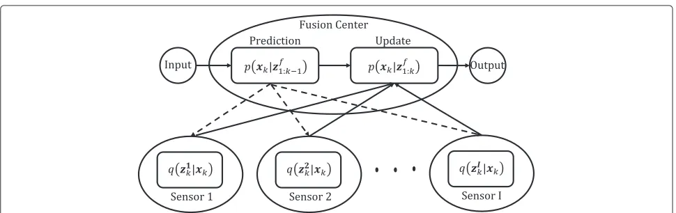
Then, our distributed architecture is obtained by uti-lizing (6) to decompose the computation of (4) to each sensor, which is summarized in Fig. 1.
Figure 1 shows that, in the fusion process of time step k, the fusion center makes a prediction with (3). Then, the information of prediction is sent to each distributed sensor, in which the likelihood is calculated. Afterwards, each sensor sends the likelihood back to the fusion center to yield the final result with (6). Finally, the fusion result feeds back to the fusion center as the prior information of the next step.
3 Sub-optimality in CI algorithm with feedback
structure
This section analyzes the sub-optimality of the existing CI algorithm with feedback structure, by comparing it with the aforementioned distributed fusion in Section 2. This paper only concentrates on the most common scenarios that the distribution in SSM is Gaussian [18]. Without loss of generality, the fusion withIsensors is considered, whereI≥2. According to [19], for anyw∈(0, 1), the pos-terior distribution of two sensors fusion in CI algorithm holds:
. Given (7), the posterior distribution
p
xk|zf1:k
can be derived as follows,
p according to (7) as follows
p
This completes the proof of Lemma 1.
In the feedback structure, Lemma 1 provides a general-ized form of posterior distributionpxk|zf1:k
calculated in CI fusion. As seen from (8) and (6), the CI algorithm adds a fractional powerωito each likelihood.
Lemma 2.Assuming that likelihoods obey Gaussian dis-tribution, i.e., qzik|xk andσi2is the corresponding variance. Then, the variance of likelihood in each sensor becomesσi2/ωiin CI algorithm.
Proof. According to Lemma 1, the posterior distribution of CI is calculated with (8) as
p
Hence, the variance of each likelihood in CI fusion has turned into σi2/ωi in the process of calculating
the posterior distribution. This completes the proof of Lemma 2.
Since there exists
ωi∈(0, 1)⇒σi2/ωi> σi2,
ωiincreases the variance of likelihood in CI fusion. Hence,
compared with (6) in the distributed fusion of Section 2, the estimation (8) calculated in CI contains more uncer-tainty under the same observations. Such unceruncer-tainty leads to the increment of estimation error. As a result, the sub-optimality still exists in CI fusion with feedback structure.
4 Monte Carlo Bayesian algorithm
To avoid the increment of estimation error, this paper utilizes the distributed fusion architecture in Section 2 to develop the fusion algorithm. In the most common applications, the observation is nonlinear [20]. Therefore, the posterior distributed in (6) cannot be simply calcu-lated by joint Gaussian method with the procedure of squares completion [21]. To solve this problem, our MCB algorithm is proposed. This algorithm incorporates the Monte Carlo sampling into the distributed fusion archi-tecture, by which the posterior distribution can be directly approximated with particles.
4.1 Monte Carlo sampling in MCB algorithm
At time k, N independent random particles are drawn from prediction distributionp According to the approximation inference method of numerical sampling [17], the prediction distribution p
xk|zf1:k−1
can be approximated as follows,
pxk|zf1:k−1
According to (14), the posterior distribution in (6) can be approximated as,
whereCis the normalization constant.
4.2 Fusion with MCB algorithm
According to the distributed fusion architecture in section 2, the estimation of statexkis calculated iteratively
by (3) and (6).
First, in the fusion center, at time stepk, given the pre-vious state estimation with the meanx¯k−1 and variance
Pk−1, the unscented sigma point setχk−1is calculated as
point set, andλis the scaling parameter [22]. Then, the prediction (3) is calculated in the form of meanx¯k|k−1and
wheref(·)is the state transition function,Qis the variance of corresponding noise,Wim ∈ Wm andWic ∈ Wcare unscented transformation parameters calculated before estimation [22]. Then, N particles are drawn from the Gaussian approximation of prediction:
{Xnk ∼N(xk; x¯k|k−1, Pk|k−1)}Nn=1.
Second, the particles are sent to each sensor node. After achieving the observationzik in the ith sensor, the likeli-hood is approximated by the set: qzik|XnkNn=1. Then, each sensor sends its own approximated likelihood back to the fusion center.
¯
In this section, the simulation results are provided to validate the performance of our MCB algorithm. In our simulation, a classic two-dimensional (2-D) fusion sce-nario with the nonlinear observation of one active and two passive radars is considered. In such a scenario, the fusion process is simulated by tracking a single target under sev-eral cases. For each case, different noise and kinematic models of transition equation are applied. Finally, 100 Monte Carlo simulations have been run for each case, and the fusion performance of nonlinear tracking is compared between our MCB algorithm and the UKF-SCI algorithm [12] with feedback structure. Note that, in this paper, we concentrate on Gaussian tracking scenarios, in which the UKF-SCI outperforms the DPF-ICI [13].
5.1 Simulation setup
In the common radar system, the transition Eq. (1) is considered as
xk=Fxk−1+nk−1, (22)
wherexk =[dx,k, dy,k, vx,k, vy,k]Tis the column vector,
indicating the 2-D distance and velocity of a single target in thex−yplane at time stepk.Fis the state transition matrix with sampling intervalsT. In this paper, three state
transition matrices are taken into account for three kine-matic models: constant-velocity (CV) and constant-turn (CT) with known turn ratesω=2.5◦/sandω=5◦/s[23]:
for CT model [24]. The trajectories of three kinematic models in our scenario are shown in Fig. 2.
In addition, nk =[nd, nd, nv, nv]T represents the
state transition noise in distance and velocity. For fair comparison, this paper utilizes the same noise for differ-ent models which obeys the Gaussian distribution, i.e., nd ∼ N(nd; 0,σd2) andnv ∼ N(nv; 0,σv2). Here,σd and
σv=2σd/sT are standard deviations of transition noise of
distance and velocity, respectively.
In our simulation, the observation equation in (2) is replaced by active and passive radar observation equations defined as,
Passive:zk=arctan
dy,k
dx,k +nθ, (26)
wherenθ ∼ N(nθ; 0,σθ2), nr ∼ N(nr; 0,σr2); σθ andσr
are standard deviations for tracking azimuth and distance. Then, we evaluate the performance of fusion with three radars, i.e., one active and two passive radars. Follow-ing [25], the aforementioned parameters are set assT =
0.1(s), σθ = 0.0001(rad), σr = 0.5(m), and σd =
{0.25, 0.3, 0.35, 0.4}(m).
The simulation setting may be applied to a compos-ite guidance scenario [26], in which there are one active and two passive radars [27, 28]. Although we simplify the observation equation in a 2-D scenario, the simula-tion scenario is still suitable for the practical applicasimula-tion of tracking and surveillance in network centric warfare (NCW) [29].
5.2 Evaluation
(a) (b)
(c)
Fig. 2The trajectories of target for three dynamic models. There are three sub-figuresa,b, andcin this figure.ais the trajectory drew according CV model.bis the trajectory drew according CT model with turn rateω=2.5◦/s.cis the trajectory drew according CT model with turn rateω=5◦/s
(a) (b)
(c) (d)
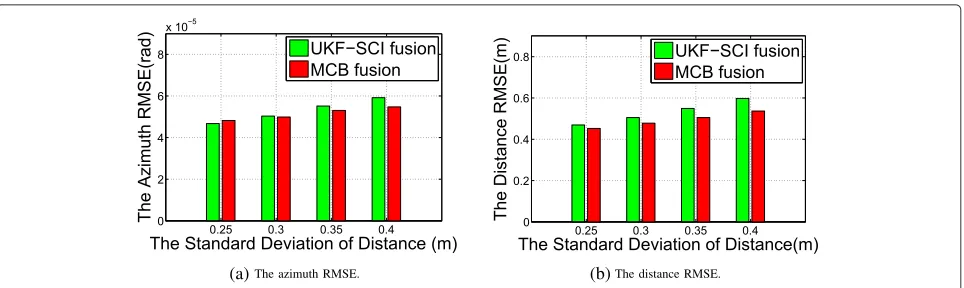
(a) (b)
Fig. 4The comparison of azimuth and distance RMSE at different standard deviations of distance, with CV model. There are two sub-figuresaandb in this figure, in which, under the CV model, the changes of fusion RMSE of azimuth and distance are described along with different standard deviations of distance. The fusion RMSE inaandbis the mean of all results covering all fusion time steps
The simulation results of CV model are shown in Figs. 3 and 4. In Fig. 3, two scenarios with σd = {0.3, 0.4}
are selected to show the fusion root-mean-squared-error (RMSE) averaged over all 100 Monte Carlo simulations, along with the tracking time. Obviously, we can see from Fig. 3 that our MCB algorithm reduces the RMSE of both azimuth and distance, along with the tracking time.
Such RMSE reduction becomes larger, when the transi-tion noise increases. Furthermore, in Fig. 4, we show the average RMSE (from tracking time 3 to 50 s) of MCB and UKF-SCI algorithms with all scenarios of four transition noises. As seen from this figure, our MCB algorithm out-performs the UKF-SCI algorithm in all cases except the azimuth case ofσd = 0.25. In addition, the improvement
(a) (b)
(c) (d)
Fig. 5The fusion RMSE of azimuth and distance for both MCB and UKF-SCI algorithms, with CT model of turn rate 2.5◦/s. In the upper figures,
(a) (b)
Fig. 6The comparison of azimuth and distance RMSE at different standard deviations of distance, with CT model of turn rate 2.5◦/s. There are two sub-figures (a) and (b) in this figure, in which, under the CT model of turn rate 2.5◦/s., the changes of fusion RMSE of azimuth and distance are described along with different standard deviations of distance. The fusion RMSE in (a) and (b) is the mean of all results covering all fusion time steps
of our MCB algorithm increases, when the transition noise becomes larger.
The simulation results of CT model are shown in Figs. 5, 6, 7, and 8. Figures 5 and 6 show the fusion RMSE com-parison of MCB and UKF-SCI algorithms with the known turn rateω=2.5◦/s. Figures 7 and 8 show the same things with the known turn rateω=5◦/s. All the results in these
figures are similar to the ones in Figs. 3 and 4. Hence, our MCB algorithm also outperforms the UKF-SCI algorithm with CT models. In addition, our MCB algorithm can per-form better when the turn rate increases. The details are shown in Tables 2 and 3.
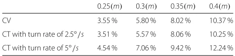
Tables 2 and 3 depict the proportions of reduced RMSE for different kinematic models and noises. As seen in
Fig. 7The fusion RMSE of azimuth and distance for both MCB and UKF-SCI algorithms, with CT model of turn rate 5◦/s. In the upper figures,
Fig. 8The comparison of azimuth and distance RMSE at different standard deviations of distance, with CT model of turn rate 5◦/s. There are two sub-figures (a) and (b) in this figure, in which, under the CT model of turn rate 5◦/s., the changes of fusion RMSE of azimuth and distance are described along with different standard deviations of distance. The fusion RMSE in (a) and (b) is the mean of all results covering all fusion time steps
these two tables, the reduction of RMSE becomes larger when the transition noise increases. This is consistent with the results shown in aforementioned figures. More-over, the reduction of RMSE with CT model of turn rate 5◦/s is largest among all three kinematic models. That means, our MCB algorithm has more advantage for high maneuvering targets.
In summary, based on the BTF, our MCB algorithm makes full use of the information of all observations, and fuses it to obtain more accurate estimation on target track-ing. Hence, compared with the CI algorithm, there are two advantages in our MCB algorithm: (1) When the tran-sition noise is large, the fusion RMSE of azimuth and distance is still small; (2) When the turn rate is large, the fusion RMSE of azimuth and distance is small as well. In other words, in the high maneuvering cases such as large transition noise and turn rate, our MCB outperforms the state-of-the-art CI algorithm, in terms of the fusion RMSE.
5.3 Computational complexity
In this section, the computational complexity of our MCB algorithm is analysed. According to Section 4.2, in the fusion center, the algorithm contains two steps for each iteration: the prediction and update steps. In the prediction step, according to (18) and (19), the mean and variance are calculated with a summed form, in which the computational complexity is proportional to
Table 2The proportion of azimuth RMSE reduced by MCB algorithm over UKF-SCI, with four standard deviations of transition noise
0.25(m) 0.3(m) 0.35(m) 0.4(m)
CV −2.51 % 1.29 % 4.90 % 7.78 %
CT with turn rate of 2.5◦/s −3.19 % 0.88 % 4.10 % 7.43 % CT with turn rate of 5◦/s −0.53 % 3.47 % 7.47 % 10.36 %
the dimension of tracking state. Moreover,Nparticles are drawn by sampling precess whose complexity is O(N). In the update step, firstly, we need to multiple allIsensors information of each particle to form a fusion likelihood. The computational complexity of this process is O(I). Then, the likelihood is used to compute the fusion results with the complexity being O(N), according to (20) and (21). In summary, the computational complexity in the update step is O(I·N).
To further evaluate the computational complexity of our MCB algorithm, we have recorded the computational time of the prediction and update steps, respectively, for one iteration in the simulation. Specially, the computer used for the test is with Intel Core i7-3770 CPU at 3.4 GHz and 4 GB RAM. In the aforementioned tracking case in Sections 5.1 and 5.2, the dimension of tracking state is 4, the particle number is 200 and the sensor number is 3. Through the simulation, we found out that the predic-tion and update steps take around 0.563 and 2.3 ms for one iteration. In other word, we only need 2.863 ms to compute the tracking results in the fusion center at each iteration. Hence, this algorithm is fast enough to utilize in the fields of radar tracking and fusion.
6 Conclusions
In this paper, we have proposed a novel MCB algorithm to achieve the distributed fusion estimation of nonlinear tracking. First, the distributed fusion architecture is set
Table 3The proportion of distance RMSE reduced by MCB algorithm over UKF-SCI, with four standard deviations of transition noise
0.25(m) 0.3(m) 0.35(m) 0.4(m)
CV 3.55 % 5.80 % 8.02 % 10.37 %
up based on BTF. Second, the sub-optimality in CI algo-rithms is proved. Then, to solve the estimation problem of nonlinear tracking, the Monte Carlo sampling method is incorporated into the distributed architecture. Benefiting from this sampling method, the approximation of fusion results is obtained through random particles. Simulation results verify that our MCB algorithm outperforms the state-of-the-art CI algorithm.
In summary, there are three directions of the future work in our paper. (1) Our MCB algorithm only offers a distributed calculation on the update step. Hence, a total distributed fusion structure is needed to further reduce the computation and communication overhead. (2) The time-discrete SSM used in our paper is actually a special case of continuous-time SSM. Therefore, we can extend our method to the exponential tracking scenario, in which the filtering can be processed with partially unknown and uncertain transition probabilities [30–33] with Markovian jump system. (3) Unknown inputs which represent the faults can be added into SSM and the residuals are cal-culated [34]. Hence, the fault detection algorithms [35] and the fuzzy model [36] can also be incorporated into our fusion system to strengthen the reliability of fusion process in the future work.
Endnote
1The feedback structure means a structure which feeds
the tracking result back to each sensor as the prior knowledge for the next step.
Competing interests
The authors declare that they have no competing interests.
Authors’ contributions
This work is a product of inputs and work of all the authors to the research concept and experiment.
Acknowledgements
This work was supported by the National Nature Science Foundation of China projects under Grants 61471022 and 61573037.
Received: 30 December 2015 Accepted: 6 May 2016
References
1. DL Hall, J Llinas, An introduction to multisensor data fusion. Proc. IEEE.
85(1), 6–23 (1997). doi:10.1109/5.554205
2. S Xu, RC de Lamare, HV Poor, Adaptive link selection algorithms for distributed estimation. EURASIP J. Adv. Signal Process.2015(1), 1–22 (2015)
3. SB Hassen, A Samet, An efficient central doa tracking algorithm for multiple incoherently distributed sources. EURASIP J. Adv. Signal Process.
2015(1), 1–19 (2015)
4. Y Bar-Shalom, L Campo, The effect of the common process noise on the two-sensor fused-track covariance. Aerosp. Electron. Syst. IEEE Trans.
AES-22(6), 803–805 (1986). doi:10.1109/TAES.1986.310815 5. KC Chang, RK Saha, Y Bar-Shalom, M Alford, inMultisensor Fusion and
Integration for Intelligent Systems, 1996. IEEE/SICE/RSJ International Conference On. Performance evaluation of multisensor track-to-track fusion (IEEE, Washington, DC, 1996), pp. 627–632.
doi:10.1109/MFI.1996.572239
6. XR Li, Y Zhu, J Wang, C Han, Optimal linear estimation fusion .i. unified fusion rules. Inf. Theory IEEE Trans.49(9), 2192–2208 (2003). doi:10.1109/TIT.2003.815774
7. T Wang, Y Zhang, J Qiu, H Gao, Adaptive fuzzy backstepping control for a class of nonlinear systems with sampled and delayed measurements. IEEE Trans. Fuzzy Syst.23(2), 302–312 (2015)
8. T Wang, H Gao, J Qiu, A combined adaptive neural network and nonlinear model predictive control for multirate networked industrial process control. IEEE Trans. Neural Netw. Learn. Syst.27(99), 416–425 (2015) 9. T Wang, H Gao, J Qiu, A combined fault-tolerant and predictive control
for network-based industrial processes. IEEE Trans. Ind. Electron.
63, 1–1 (2016)
10. SJ Julier, JK Uhlmann, inAmerican Control Conference, 1997. Proceedings of the 1997. A non-divergent estimation algorithm in the presence of unknown correlations, vol. 4 (IEEE, Albuquerque, NM, 1997), pp. 2369–23734. doi:10.1109/ACC.1997.609105
11. M Reinhardt, B Noack, PO Arambel, UD Hanebeck, Minimum covariance bounds for the fusion under unknown correlations. Signal Process. Lett. IEEE.22(9), 1210–1214 (2015)
12. Z Deng, P Zhang, W Qi, J Liu, Y Gao, Sequential covariance intersection fusion kalman filter. Inf. Sci.189, 293–309 (2012)
13. O Hlinka, O Sluciak, F Hlawatsch, M Rupp, inAcoustics, Speech and Signal Processing (ICASSP), 2014 IEEE International Conference On. Distributed data fusion using iterative covariance intersection (IEEE, Florence, 2014), pp. 1861–1865
14. SJ Julier, inTarget Tracking and Data Fusion: Algorithms and Applications, 2008 IET Seminar On. Fusion without independence (IET, Birmingham, 2008), pp. 1–1
15. S Mori, KC Chang, CY Chong, inInformation Fusion (FUSION), 2012 15th International Conference On. Comparison of track fusion rules and track association metrics (IEEE, 2012), pp. 1996–2003
16. A Doucet, X Wang, Monte carlo methods for signal processing: a review in the statistical signal processing context. Signal Process. Mag. IEEE.
22(6), 152–170 (2005). doi:10.1109/MSP.2005.1550195
17. CM Bishop,Pattern recognition and machine learning (information science and statistics). (Springer, New York, 2006), pp. 523–524
18. T Song, H Kim, D Musicki, Distributed (nonlinear) target tracking in clutter. Aerosp. Electron. Syst. IEEE Trans.51(1), 654–668 (2015)
19. MB Hurley, inInformation Fusion, 2002. Proceedings of the Fifth International Conference On. An information theoretic justification for covariance intersection and its generalization, vol. 1 (IEEE, Annapolis, MD, USA, 2002), pp. 505–5111. doi:10.1109/ICIF.2002.1021196
20. Y He, JJ Xiu, JW Zhang, X Guan,Radar Data Processing with Applications. (Beijing: Publishing house of electronics industry, Beijing, 2006) 21. A Doucet, S Godsill, C Andrieu, On sequential Monte Carlo sampling
methods for Bayesian filtering. Stat. Comput.10(3), 197–208 (2000) 22. R Van Der Merwe, A Doucet, N De Freitas, E Wan, inNIPS. The unscented
particle filter (MIT press, Cambridge, MA, 2000), pp. 584–590 23. XR Li, Y Bar-Shalom, Design of an interacting multiple model algorithm
for air traffic control tracking. Control Syst. Technol. IEEE Trans.1(3), 186–194 (1993)
24. XR Li, VP Jilkov, Survey of maneuvering target tracking. part i. dynamic models. Aerosp. Electron. Syst. IEEE Trans.39(4), 1333–1364 (2003) 25. Y He, G Wang, X Guan,Information Fusion Theory With Applications.
(Publishing House of Electronics Industry, Beijing, 2010) 26. B Fan, YL Qin, JT Wang, HT Xiao, in2011 International Workshop on
Multi-Platform/Multi-Sensor Remote Sensing and Mapping. 3d multiple maneuvering targets tracking in active and passive radar composite guidance, (2011), pp. 1–6
27. Q He, J Hu, RS Blum, Y Wu, Generalized cramer rao bound for joint estimation of target position and velocity for active and passive radar networks. IEEE Trans. Signal Process.64(8), 2078–2089 (2016) 28. YD Zhang, MG Amin, B Himed, Joint dod/doa estimation in mimo radar
exploiting time-frequency signal representations. J. Adv. Signal Process.
2012(1), 1–10 (2012)
29. D Smith, S Singh, Approaches to multisensor data fusion in target tracking: a survey. Knowle. Data Eng. IEEE Trans.18(12), 1696–1710 (2006) 30. Y Wei, J Qiu, HR Karimi, M Wang,H∞model reduction for
31. Y Wei, J Qiu, HR Karimi, M Wang, Filtering design for two-dimensional markovian jump systems with state-delays and deficient mode information. Inf. Sci.269(4), 316–331 (2014)
32. Y Wei, J Qiu, HR Karimi, M Wang, A new design ofH∞filtering for continuous-time markovian jump systems with time-varying delay and partially accessible mode information. Signal Process.93(9), 2392–2407 (2013)
33. J Qiu, Y Wei, HR Karimi, New approach to delay-dependentH∞control for continuous-time markovian jump systems with time-varying delay and deficient transition descriptions. J. Frankl. Inst.352(1), 189–215 (2015) 34. L Li, SX Ding, J Qiu, Y Yang, Weighted fuzzy observer-based fault detection
approach for discrete-time nonlinear systems via piecewise-fuzzy lyapunov functions. IEEE Trans. Fuzzy Syst. (99), 1–13 (2016) 35. L Li, SX Ding, J Qiu, Y Yang, Real-time fault detection approach for
nonlinear systems and its asynchronous t-s fuzzy observer-based implementation. Cybernet. IEEE Trans. (99), 1–12 (2016)
36. J Qiu, S Ding, H Gao, S Yin, Fuzzy-model-based reliable static output feedback h-infinity control of nonlinear hyperbolic pde systems. IEEE Trans. Fuzzy Syst.24(2), 388–400 (2015)
Submit your manuscript to a
journal and benefi t from:
7Convenient online submission 7Rigorous peer review
7Immediate publication on acceptance 7Open access: articles freely available online 7High visibility within the fi eld
7Retaining the copyright to your article