alternating direction method of multipliers
Gui-Bo Ye Yifei Chen Xiaohui Xie
University of California, Irvine University of California, Irvine University of California, Irvine
Abstract
The support vector machine (SVM) is a widely used tool for classification. Although commonly understood as a method of find-ing the maximum-margin hyperplane, it can also be formulated as a regularized func-tion estimafunc-tion problem, corresponding to a hinge loss function plus an ℓ2-norm reg-ulation term. The doubly regularized sup-port vector machine (DrSVM) is a variant of the standard SVM, which introduces an ad-ditional ℓ1-norm regularization term on the fitted coefficients. The combined ℓ1 and ℓ2regularization, termed elastic net penalty, has the property of achieving simultaneous variable selection and margin-maximization within a single framework. However, because of the nondifferentiability of both the loss function and the regularization term, there is no efficient method available to solve DrSVM for large-scale problems. Here we develop an efficient algorithm based on the alternating direction method of multipliers (ADMM) to solve the optimization problem in DrSVM. The utility of the method is illustrated using both simulated and real-world data.
1 INTRODUCTION
Datasets with tens of thousands variables have become increasingly common in many real-world applications. For example, in the biomedical domain a microarray dataset typically contains about 20,000 genes, while a genotype dataset commonly includes half of a million SNPs. Regularization terms that encourage sparsity in coefficients are increasingly being used for simul-Appearing in Proceedings of the 14𝑡ℎ International Con-ference on Artificial Intelligence and Statistics (AISTATS) 2011, Fort Lauderdale, FL, USA. Volume 15 of JMLR: W&CP 15. Copyright 2011 by the authors.
taneous variable selection and prediction (Tibshirani, 1996; Zou and Hastie, 2005).
A widely used strategy for imposing sparsity on regres-sion or classification coefficients is to use theℓ1-norm regularization. Perhaps the most well-known example is the least absolute shrinkage and selection operator (lasso) method for linear regression. The method min-imizes the usual sum of squared errors while penalizing the ℓ1 norm of the regression coefficients (Tibshirani, 1996). Due to the nondifferentiability of theℓ1 norm, lasso is able to perform continuous shrinkage and auto-matic variable selection simultaneously. Although the lasso method has shown success in many situations and has been generalized for different settings (Zhu et al., 2003; Lin and Zhang, 2006), it has several limitations. First, when the dimension of the data (𝑝) is larger than the number of training samples (𝑛), lasso selects at most 𝑛 variable before it saturates (Efron et al., 2004). Second, if there is a group of variables among which the pairwise correlations are very high, the lasso tends to select only one variable from the group and does not care which one is selected.
The elastic net penalty proposed by Zou et al. in Zou and Hastie (2005) is a convex combination of the lasso and ridge penalty, which has the characteristics of both the lasso and ridge regression in the regression setting. More specifically, the elastic net penalty simultane-ously does automatic variable selection and continu-ous shrinkage, and it can select groups of correlated variables. It is especially useful for “large 𝑝, small𝑛” problems, where the “grouped variables” situation is a particularly important concern and has been addressed many times in the literature (Hastie et al., 2000, 2003). The idea of using ℓ1-norm constraints to automati-cally select variables has also been extended to classi-fication problems. Zhu et al. (2003) proposed an ℓ1-norm support vector machine, whereas Wang et al. (2006) proposed a SVM with the elastic net penalty term, which they named doubly regularized support vector machine (DrSVM). By using a mixture of the ℓ1-norm and theℓ2-norm penalties, DrSVM is able to perform automatic variable selection as the ℓ1-norm
SVM. Additionally, it also encourages highly corre-lated variables to be selected (or removed) together, and thus achieves the grouping effect.
Although DrSVM has a number of desirable features, solving DrSVM is, however, non-trivial because of the nondifferentiability in both the loss function and the regularization term. This is especially problematic for large scale problems. To circumvent this diffi-culty, Wang et al. (2008) proposed a hybrid huberized support vector machine (HHSVM), which uses a hu-berized hinge loss function to approximate the hinge loss in DrSVM. Because the huberized hinge loss func-tion is differentiable, HHSVM is easier to solve than DrSVM. Wang et al. (2008) proposed a path algorithm to solve the HHSVM problem. However, because the path algorithm requires tracking disappearance of vari-ables along a regularization path, it is not easy to im-plement and still does not handle large-scale data well. Our main contribution in this paper is to introduce a new algorithm to directly solve DrSVM without re-sorting to approximation as in HHSVM. Our method is based on the alternating direction method of mul-tipliers (ADMM) (Gabay and Mercier, 1976; Glowin-ski and Marroco). We demonstrate that the method is efficient even for large-scale problems with tens of thousands variables.
The rest of the paper is organized as follows. In Sec-tion 2, we provide a descripSec-tion of the SVM model with elastic net penalty. In Section 3, we derive an iterative algorithm based on ADMM to solve the optimization problem in DrSVM and prove its convergence prop-erty. In Section 4, we benchmark the performance of the algorithm on both simulated and real-world data.
2 SUPPORT VECTOR MACHINES
WITH ELASTIC NET PENALTY
2.1 SVM as regularized function estimation Consider the classification of the training data {(x𝑖, 𝑦𝑖)}𝑛𝑖=1, where x𝑖 = (𝑥𝑖1, . . . , 𝑥𝑖𝑝)𝑇 are the pre-dictor variables and 𝑦𝑖 ∈ {−1,1} is the correspond-ing class label. The support vector machine (SVM) was originally proposed to find the optimal separat-ing hyperplane that separates the two classes of data points with the largest margin (Vapnik, 1998). It can be equivalently reformulated as an ℓ2-norm penalized optimization problem: min 𝛽0,𝛽 1 𝑛 𝑛 ∑ 𝑖=1 (1−𝑦𝑖(𝛽0+x𝑇𝑖 𝛽))++𝜆2∥𝛽∥22, (1) where the loss function (1−⋅)+:= max(1−⋅,0) is called thehinge loss, and𝜆≥0 is a regularization parameter,which controls the balance between the ‘loss’ and the ‘penalty’.
By shrinking the magnitude of the coefficients, theℓ2 norm penalty in (1) reduces the variance of the esti-mated coefficients, and thus can achieve better pre-diction accuracy. However, the ℓ2 norm penalty can-not produce sparse coefficients and hence cancan-not au-tomatically perform variable selection. This is a ma-jor limitation for applying SVM to do classification in some high-dimensional data, such as gene expression data from microarrays (Guyon et al., 2002; Mukherjee et al., 1999), where variable selection is essential for both achieving better prediction accuracy and provid-ing reasonable interpretations.
To include variable selection, Zhu et al. (2003) pro-posed anℓ1-norm support vector machine,
min 𝛽0,𝛽 1 𝑛 𝑛 ∑ 𝑖=1 (1−𝑦𝑖(𝛽0+x𝑇𝑖𝛽))++𝜆∥𝛽∥1, (2) which do variable selection automatically via the ℓ1 penalty. However, it shares similar disadvantages as the lasso method for ‘large𝑝, small𝑛’ problems, such as selecting at most 𝑛 relevant variables, and disre-garding group effects. This is not satisfying for some application problems. In microarray analysis, we al-most always have 𝑝 ≫𝑛. Furthermore, the genes in the same biological pathway frequently show highly correlated expression; it is desirable to identify all, in-stead a subset, of them for both providing biological interpretations and building prediction models. One natural way to overcome the limitations outlined above is to apply the elastic net penalty to the SVM:
min 𝛽0,𝛽 1 𝑛 𝑛 ∑ 𝑖=1 (1−𝑦𝑖(𝛽0+x𝑇𝑖𝛽))++𝜆1∥𝛽∥1+𝜆22∥𝛽∥22, (3) where 𝜆1, 𝜆2 ≥0 are regularization parameters. The model was originally proposed by Wang et al. (2006), and was named doubly regularized SVM (DrSVM). However, to emphasize the role of elastic net penalty, we refer to this model (3) as elastic net SVM or simply ENSVM in the rest of the paper. Due to the properties of the elastic net penalty, the optimal solution of (3) will enjoy both the sparse and the grouping effect the same as the elastic net method in regression.
2.2 RELATED WORK
A similar model has been proposed by Wang et al. (2008) who have applied the elastic net penalty to the huberized hinge function and proposed the HHSVM:
min 𝛽0,𝛽 1 𝑛 𝑛 ∑ 𝑖=1 𝜙(𝑦𝑖(𝛽0+x𝑇𝑖𝛽)) +𝜆1∥𝛽∥1+𝜆22∥𝛽∥22, (4)
where 𝜙is the huberized hinge loss function: 𝜙(𝑡) = ⎧ ⎨ ⎩ 0, for𝑡 >1, (1−𝑡)2/2𝛿, for 1−𝛿 < 𝑡≤1, 1−𝑡−𝛿/2, for𝑡≤1−𝛿 (5)
with 𝛿 > 0 being a pre-specified constant. The main motivation for Wang et al. (2008) to use huberized hinge loss function (5) is that it is an approximation of the hinge loss and differentiable everywhere, thereby making the optimization problem easier to solve while at the same time preserving the variable selection fea-ture.
The minimizer of (4) is piecewise linear with respect
to 𝜆1 for a fixed 𝜆2. Based on this observation, Wang
et al. (2008) proposed a path algorithm to solve the HHSVM problem. The path algorithm keeps track of
four sets as𝜆1decreases, and calls an ’event’
happen-ing if any one of the four sets changes. Between any
two consecutive ’events’, the solutions are linear in𝜆1,
and after an ’event’ occurs, the derivative of the
solu-tion with respect to 𝜆1 is changed. When each ’event’
happens, the algorithm solves a linear system. If the
dimension of the data 𝑝 is large, solving many
large-scale linear systems will be required to obtain the so-lution path. Furthermore, those linear equations are quite different from each other, and there are no special structures involved. As a result, the path algorithm is
computational very expensive for large 𝑝problems.
3 ALGORITHM FOR ELASTIC
NET SVM
The alternating direction method of multipliers (ADMM) developed in the 1970s (Gabay and Mercier, 1976; Glowinski and Marroco) has recently become a method of choice for solving many large-scale prob-lems (Candes et al., 2009; Cai et al., 2009; Goldstein and Osher, 2009). It is equivalent or closely related to many other algorithms, such as Douglas-Rachford splitting (Wu and Tai, 2010), split Bregman method (Goldstein and Osher, 2009) and the method of mul-tipliers (Rockafellar, 1973).
In this section, we propose an efficient algorithm based on ADMM to solve ENSVM in (3) by introducing aux-iliary variables and reformulating the original problem.
3.1 DERIVING ADMM FOR ELASTIC NET SVM
Because of the two nondifferentiable terms in (3), it is hard to solve the ENSVM problem directly. In or-der to or-derive an ADMM algorithm, we introduce some auxiliary variables to handle the nondifferentiability of
the hinge loss andℓ1norm term.
Let 𝑋 = (𝑥𝑖𝑗)𝑛,𝑝𝑖=1,𝑗=1 and 𝑌 be a diagonal matrix
with its diagonal elements to be the vector 𝑦 =
(𝑦1, . . . , 𝑦𝑛)𝑇. The unconstrained problem in (3) can
be reformulated into an equivalent constrained prob-lem arg min 𝛽,𝛽0 1 𝑛 𝑛 ∑ 𝑖=1 (𝑎𝑖)++𝜆1∥c∥1+𝜆22∥𝛽∥22 𝑠.𝑡. a=1−𝑌 (𝑋𝛽+𝛽01), c=𝛽, (6)
where a = (𝑎𝑖, . . . , 𝑎𝑛)𝑇 and1is an 𝑛-column vector
of 1s.
Note that the Lagrangian function of (6) is
𝐿(𝛽, 𝛽0,a,c,u,v) = 1𝑛 𝑛 ∑ 𝑖=1 (𝑎𝑖)++𝜆1∥c∥1+𝜆22 ∥𝛽∥22 +⟨u,1−𝑌(𝑋𝛽+𝛽01)−a⟩+⟨v, 𝛽−c⟩,(7)
where u∈ℝ𝑛 is a dual variable corresponding to the
linear constraint a = 1−𝑌 (𝑋𝛽+𝛽01), v ∈ ℝ𝑝 is
a dual variable corresponding to the linear constraint
c = 𝛽, ⟨⋅,⋅⟩ denotes the standard inner product in
Euclidean space. The augmented Lagrangian func-tion of (6) is similar to (7) except for adding two
terms 𝑢1
2∥1−𝑌 (𝑋𝛽+𝛽01)−a∥22 and 𝑢22∥𝛽 −c∥22
to penalize the violation of linear constraints a =
1−𝑌 (𝑋𝛽+𝛽01) andc=𝛽, thereby making the
func-tion strictly convex. That is,
ℒ(𝛽, 𝛽0,a,c,u,v)
= 𝐿(𝛽, 𝛽0,a,c,u,v) +𝜇21∥1−𝑌(𝑋𝛽+𝛽01)−a∥22
+𝜇22∥𝛽−c∥2
2, (8)
where𝜇1>0 and𝜇2>0 are two parameters. It is easy
to see that solving (6) is equivalent to finding a saddle point (𝛽∗, 𝛽∗ 0,a∗,c∗,u∗,v∗) ofℒ(𝛽, 𝛽0,a,c,u,v) such that ℒ(𝛽∗, 𝛽∗ 0,a∗,c∗,u,v) ≤ ℒ(𝛽∗, 𝛽0∗,a∗,c∗,u∗,v∗) ≤ ℒ(𝛽, 𝛽0,a,c,u∗,v∗),
for all𝛽, 𝛽0,a,c,uandv.
We solve the saddle point problem through gradient ascent on the dual problem
max
u,v 𝐸(u,v), (9)
where 𝐸(u,v) = min𝛽,𝛽0,a,cℒ(𝛽, 𝛽0,a,c,u,v). Note
that the gradient ∇𝐸(u,v) can be calculated by the
following (Bertsekas, 1982) ∇𝐸(u,v) = ( 1−𝑌(𝑋𝛽(u,v) +𝛽0(u,v)1)−a(u,v) 𝛽(u,v)−c(u,v) ) , (10)
with
(𝛽(u,v), 𝛽0(u,v),a(u,v),c(u,v))
= arg min
𝛽,𝛽0,a,cℒ(𝛽, 𝛽0,a,c,u,v). (11) Using gradient ascent on the dual problem (9), Eq. (10) and Eq. (11), we get the method of multipliers (Rockafellar, 1973) to solve (6) ⎧ ⎨ ⎩ (𝛽𝑘+1, 𝛽𝑘+1 0 ,a𝑘+1,c𝑘+1) = arg min𝛽,𝛽0,a,cℒ(𝛽, 𝛽0,a,c,u𝑘,v𝑘) u𝑘+1=u𝑘+𝜇1(1−𝑌(𝑋𝛽𝑘+1+𝛽𝑘+1 0 1)−a𝑘+1), v𝑘+1=v𝑘+𝜇 2(𝛽𝑘+1−c𝑘+1). (12) The efficiency of the iterative algorithm (12) lies on whether the first equation of (12) can be solved quickly. The augmented Lagrangian function ℒ still contains nondifferentiable terms. But different from the original objective function (3), the hinge loss in-duced nondifferentiability has now been transferred from terms involving 1−𝑦𝑖(x𝑇𝑖𝛽 +𝛽0) to terms
in-volving𝑎𝑖; andℓ1induced nondifferentiability has now
been transferred from terms involving 𝛽 to terms in-volving c. Moreover, the nondifferentiable terms in-volving a and c are now completely decoupled, and thus we can solve the first equation of (12) by alter-nating minimization of (𝛽, 𝛽0),aandc,
⎧ ⎨ ⎩ (𝛽𝑘+1, 𝛽𝑘+1 0 ) = arg min𝛽,𝛽0ℒ(𝛽, 𝛽0,a𝑘,c𝑘,u𝑘,v𝑘), a𝑘+1= arg min aℒ(𝛽𝑘+1, 𝛽0𝑘+1,a,c𝑘,u𝑘,v𝑘 ) , c𝑘+1= arg mincℒ(𝛽𝑘+1, 𝛽𝑘+1 0 ,a𝑘+1,c,u𝑘,v𝑘 ) . (13) For the method of multipliers, the alternate minimiza-tion (13) needs to run multiple times until conver-gence. However, we do not have to completely solve the first equation of (12) since it is only one step of the overall iterative algorithm. We use only one al-ternation, it is called alternating direction method of multipliers (Gabay and Mercier, 1976). That is, we use the following iterations to solve (6)
⎧ ⎨ ⎩ (𝛽𝑘+1, 𝛽𝑘+1 0 ) = arg min𝛽,𝛽0ℒ(𝛽, 𝛽0,a𝑘,c𝑘,u𝑘,v𝑘), a𝑘+1= arg min aℒ(𝛽𝑘+1, 𝛽0𝑘+1,a,c𝑘,u𝑘,v𝑘 ) , c𝑘+1= arg mincℒ(𝛽𝑘+1, 𝛽𝑘+1 0 ,a𝑘+1,c,u𝑘,v𝑘 ) , u𝑘+1=u𝑘+𝜇 1(1−𝑌(𝑋𝛽𝑘+1+𝛽0𝑘+11)−a𝑘+1), v𝑘+1=v𝑘+𝜇 2(𝛽𝑘+1−c𝑘+1). (14)
For the first equation in (14), it is equivalent to (𝛽, 𝛽0) = arg min𝛽,𝛽0 𝜆22∥𝛽∥22+ 〈 v𝑘, 𝛽−c𝑘〉 +〈u𝑘,1−𝑌(𝑋𝛽+𝛽01)−a𝑘〉 +𝜇21∥1−𝑌(𝑋𝛽+𝛽01)−a𝑘∥2 2 +𝜇2 2 ∥𝛽−c𝑘∥22.
The objective function in the above minimization problem is quadratic and differentiable, and thus the optimal solution can be found by solving a set of linear equations: ( (𝜆2+𝜇2)𝐼+𝜇1𝑋𝑇𝑋 𝜇1𝑋𝑇1 𝜇11𝑇𝑋 𝜇1𝑛 ) ( 𝛽𝑘+1 𝛽𝑘+1 0 ) = ( 𝑋𝑇𝑌u𝑘−𝜇1𝑋𝑇𝑌(a𝑘−1)−v𝑘+𝜇2c𝑘 1𝑇𝑌u𝑘−𝜇11𝑇𝑌(a𝑘−1) ) . (15) Note that the coefficient matrix in (15) is a (𝑝+1)×(𝑝+ 1) matrix, independent of the optimization variables. For small𝑝, we can store its inverse in the memory, so the linear equations can be solved with minimal cost. For large 𝑝, we use the conjugate gradient algorithm (CG) to solve it at each iteration efficiently.
The linear system (15) is very special for large𝑝, small
𝑛 problems in that 𝑋𝑇𝑋 will be a positive low rank
matrix with rank at most 𝑛. Thus the coefficient ma-trix in (15) is a linear combination of identity mama-trix and a positive low rank matrix with rank at most𝑛+1. If we use CG to solve the linear system (15), it con-verges in less than𝑛+1 steps (Saad, 2003). In our nu-merical implementation, we found that CG converges in a few steps much smaller than𝑛+ 1.
For the second equation in (14), it is equivalent to
a𝑘+1 = arg min a 1 𝑛 𝑛 ∑ 𝑖=1 (𝑎𝑖)+ +𝜇21∥1−𝑌(𝑋𝛽𝑘+1+𝛽𝑘+1 0 1)−a∥22 +⟨u𝑘,1−𝑌(𝑋𝛽𝑘+1+𝛽𝑘+1 0 1)−a⟩. (16) In order to solve (16), we need the following Proposi-tion (Ye and Xie, 2010).
Proposition 1 Let 𝑠𝜆(𝜔) = arg min𝑥∈ℝ𝜆𝑥++12∥𝑥− 𝜔∥2 2. Then 𝑠𝜆(𝜔) = ⎧ ⎨ ⎩ 𝜔−𝜆, 𝜔 > 𝜆 0, 0≤𝜔≤𝜆, 𝜔, 𝜔 <0.
Note that each𝑎𝑖is independent of each other in (16) and ∥u∥2 2 2𝜇1 + 𝜇1 2 ∥1−𝑌(𝑋𝛽𝑘+1+𝛽𝑘+10 1)−a∥22 +⟨u𝑘,1−𝑌(𝑋𝛽𝑘+1+𝛽𝑘+1 0 1)−a⟩ = 𝜇21∥a−(1+𝜇u 1 −𝑌(𝑋𝛽 𝑘+1+𝛽𝑘+1 0 1))∥22.
Together with Proposition 1, we can then updatea𝑘+1
in (16) according to
Corollary 1 The update ofa𝑘+1 in (16)is equivalent
to a𝑘+1=𝒮 1 𝑛𝜇1(1+ u𝑘 𝜇1 −𝑌(𝑋𝛽 𝑘+1+𝛽𝑘+1 0 1)), (17) where 𝒮𝜆(𝜔) = (𝑠𝜆(𝜔1), 𝑠𝜆(𝜔2), . . . , 𝑠𝜆(𝜔𝑛))𝑇,∀𝜔∈ℝ𝑛.
For the third equation in (14), it is equivalent to
c𝑘+1= arg min
c 𝜆1∥c∥1+⟨v
𝑘, 𝛽𝑘+1−c⟩+𝜇2
2 ∥𝛽𝑘+1−c∥22.
(18) Minimization of cin (18) can be done efficiently us-ing soft thresholdus-ing, because the objective function is quadratic and nondifferentiable terms are completely separable. Let𝒯𝜆 be a soft thresholding operator
de-fined on vector space and satisfying
𝒯𝜆(𝜔) = (𝑡𝜆(𝜔1), . . . , 𝑡𝜆(𝜔𝑝)),∀𝜔∈ℝ𝑝, (19)
where
𝑡𝜆(𝜔𝑖) = sgn(𝜔𝑖) max{0,∣𝜔𝑖∣ −𝜆}.
Using the soft thresholding operator (19), the optimal solution ofcin (18) can be written as
c𝑘+1=𝒯𝜆 1 𝜇2 ( v𝑘 𝜇2 +𝛽 𝑘+1 ) . (20)
Finally, by combining (14), (15), (17) and (20) to-gether, we obtain the algorithm ADMM for ENSVM (3) (Algorithm 1). It is a practical algorithm for large
𝑝, small𝑛problems and very easy to code.
3.2 Convergence analysis
The convergence property of Algorithm 1 can be de-rived from the standard convergence theory of the al-ternating direction method of multipliers (Gabay and Mercier, 1976; Eckstein and Bertsekas, 1992).
Algorithm 1ADMM for ENSVM (3) Initialize𝛽0, 𝛽0
0,a0,c0,u0, andv0. repeat
1) Update𝛽𝑘+1, 𝛽𝑘+1
0 by solving the following
lin-ear equation system:
( (𝜆2+𝜇2)𝐼+𝜇1𝑋𝑇𝑋 𝜇1𝑋𝑇1 𝜇11𝑇𝑋 𝜇1𝑛 ) ( 𝛽𝑘+1 𝛽0𝑘+1 ) = ( 𝑋𝑇𝑌u𝑘−𝜇 1𝑋𝑇𝑌(a𝑘−1)−v𝑘+𝜇2c𝑘 1𝑇𝑌u𝑘−𝜇 11𝑇𝑌(a𝑘−1) ) 2) a𝑘+1=𝒮 1 𝑛𝜇1 ( 1+u𝑘 𝜇1 −𝑌(𝑋𝛽 𝑘+1+𝛽𝑘+1 0 1) ) 3) c𝑘+1=𝒯𝜆 1 𝜇2 ( v𝑘 𝜇2 +𝛽 𝑘+1) 4)u𝑘+1=u𝑘+𝜇 1(1−𝑌(𝑋𝛽𝑘+1+𝛽0𝑘+11)−a𝑘+1) 5) v𝑘+1=v𝑘+𝜇 2(𝛽𝑘+1−c𝑘+1) until Convergence
Theorem 1 Suppose there exists at least one solution
(𝛽∗, 𝛽∗
0) of (3). Assume 𝜆1 > 0, 𝜆2 > 0. Then the
following property for Algorithm 1 holds:
lim 𝑘→∞ 1 𝑛 𝑛 ∑ 𝑖=1 (1−𝑦𝑖(x𝑇𝑖𝛽𝑘+𝛽0𝑘))++𝜆1∥𝛽𝑘∥1+𝜆22∥𝛽𝑘∥22 = 𝑛1 𝑛 ∑ 𝑖=1 (1−𝑦𝑖(x𝑇𝑖 𝛽∗+𝛽∗0))++𝜆1∥𝛽∗∥1+𝜆22∥𝛽∗∥22. Furthermore, lim 𝑘→∞∥(𝛽 𝑘, 𝛽𝑘 0)−(𝛽∗, 𝛽0∗)∥= 0,
whenever (3) has a unique solution.
3.3 Computational cost
The efficiency of Algorithm 1 lies mainly on whether we can quickly solve the linear equations (15). As we have described in Section 3.1, the coefficient of the lin-ear equations (15) has a special structure and thus can be efficiently solved by the conjugate gradient method for ‘large 𝑝, small𝑛’ problems. More specifically, the computational cost for solving (15) is 𝑂(𝑛2𝑝). The
number of iterations of Algorithm (1) is hard to pre-dict and it depends on the choice of 𝜇1 and 𝜇2.
Ac-cording to our experience, we only need to iterate a few hundred iterations to get a reasonable result by choosing𝜇1 and𝜇2 correctly.
Similar to our algorithm for (3), the major computa-tional cost in each iteration for HHSVM also comes from solving a linear system. However, the linear sys-tem in HHSVM has no special structures. It takes at
least 𝑂(∣𝒜∣2) with ∣𝒜∣being the number of unknown
variables. Moreover, ∣𝒜∣ can increase at each itera-tion. Furthermore, for large scale problems, it usually takes a few thousand steps for the algorithm converges. That’s why our algorithm for (3) is much faster than the path algorithm for HHSVM for large scale prob-lems.
4 NUMERICAL RESULTS
In this section, we use time trials on both simu-lated data as well as real microarray data to illus-trate the efficiency of ADMM algorithm for solving elastic net SVM (ENSVM). To evaluate the perfor-mance of ADMM for ENSVM, we also compare it with the stochastic sub-gradient method and the path algo-rithm for HHSVM. Our algoalgo-rithm and the stochas-tic sub-gradient method were implemented in Matlab, while HHSVM was implemented in R using the R code provided by the authors in (Wang et al., 2008). All algorithms were compiled on a windows platform and time trials were generated on an Intel Core 2 Duo desk-top PC (E7500, 2.93GHz).
The stopping criteria of Algorithm 1 for ENSVM is specified as follows. Let Φ(𝛽𝑘, 𝛽𝑘
0) = 1𝑛
∑𝑛
𝑖=1(1 −
𝑦𝑖(x𝑇𝑖𝛽𝑘+𝛽0𝑘))++𝜆1∥𝛽𝑘∥1+𝜆22 ∥𝛽𝑘∥22. According to
Theorem 1, lim𝑘→∞Φ(𝛽𝑘, 𝛽0𝑘) = Φ(𝛽∗, 𝛽0∗). It is
rea-sonable to terminate the algorithm when the relative change of the energy functional Φ(𝛽, 𝛽0) falls below
certain threshold𝛿. Furthermore, Algorithm 1 is solv-ing (6), linear constraints are satisfied when it con-verges. Therefore, we would expect that √1
𝑛∥1−
𝑌(𝑋𝛽𝑘 +𝛽𝑘
01)−a𝑘∥2 ≤ 𝛿 and √1𝑝∥𝛽𝑘 −c𝑘∥2 ≤ 𝛿
when we terminate the algorithm. We used 𝛿= 10−5
in our simulation, i.e., we stop Algorithm 1 whenever
𝑅𝑒𝑙𝐸:= ∣Φ(max{1𝛽𝑘, 𝛽0𝑘,)Φ(−𝛽Φ(𝑘, 𝛽𝛽∗𝑘, 𝛽0∗)∣ 0)} ≤10 −5, 1 √ 𝑛∥1−𝑌(𝑋𝛽𝑘+𝛽0𝑘1)−a𝑘∥2≤10−5 and 1 √𝑝∥𝛽𝑘−c𝑘∥ 2≤10−5.
Note that the convergence of Algorithm 1 is guaran-teed no matter what values of 𝜇1 and𝜇2 are used as
shown in Theorem 1. However, the speed of the algo-rithm can be influenced by the choices of𝜇1and𝜇2as
it would affect the number of iterations involved. In our implementation, we found empirically that choos-ing 𝜇1= 100𝑛 and𝜇2 ∈[25,100] works well for all the
problems we tested, though the parameter selecting procedure can certainly be further improved.
4.1 SIMULATION
We consider a binary classification problem in which the sample data are lying in a𝑝dimensional space with only the first 10 dimensions being relevant for classifi-cation and the remaining variables being noises. More specifically, we generate 𝑛samples with half from +1 and the other half from−1 class. For the samples from
Table 1:
Run times (CPU seconds) of various sizes𝑝and𝑛, different correlation𝜌between the features. Methods are ADMM al-gorithm for elastic-net SVM (ENSVM), path alal-gorithm for HHSVM and stochastic sub-gradient method (SSG). The results for ENSVM and stochastic sub-gradient method are averaged over 25 runs (using 25 different values of𝜆1, 𝜆2) and the ones for HHSVM are averaged over 5 runs (using 5 different values of𝜆2). n, p Method 𝜌= 0 𝜌= 0.8 n=50 ENSVM 0.41 0.31 HHSVM 3.30 3.19 p=300 SSG 2.35 4.06 n=100 ENSVM 1.19 0.71 HHSVM 21.65 21.01 p=500 SSG 4.34 4.06 n=200 ENSVM 3.60 3.75 HHSVM 405.9 390.1 p=1000 SSG 35.40 26.86 n=300 ENSVM 14.73 16.74 HHSVM 2.07 hours 2.03 hours p=2000 SSG 123.22 122.84 n=400 ENSVM 48.62 57.15 HHSVM >6 hours >6 hours p=5000 SSG 301.10 290.15 n=500 ENSVM 144.69 170.52 HHSVM - -p=10000 SSG 785.57 909.92 +1 class, they are i.i.d drawn from a normal distribu-tion with mean
𝜇+ = (1| {z }, . . . ,1 10 ,0| {z }, . . . ,0 𝑝−10 )𝑇 and covariance Σ = ( Σ∗ 10×10 010×(𝑝−10) 0(𝑝−10)×10 𝐼(𝑝−10)×(𝑝−10) ) ,
where the diagonal elements of Σ∗ are 1 and the
off-diagonal elements are all equal to𝜌. The−1 class has a similar distribution except that
𝜇−= (−1| , . . . ,{z −1}
10
,0| {z }, . . . ,0
(𝑝−10)
So the Bayes optimal classification rule depends on
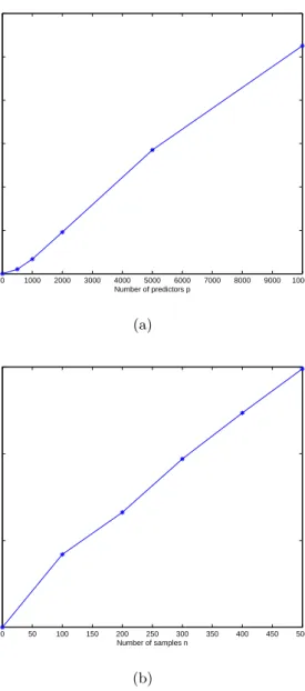
𝑥1, . . . , 𝑥10, which are highly correlated if 𝜌 is large. The Bayes error is independent of the dimension 𝑝. This simulated data were also used in Wang et al. (2008). 0 1000 2000 3000 4000 5000 6000 7000 8000 9000 10000 0 10 20 30 40 50 60 Number of predictors p CPU seconds (a) 0 50 100 150 200 250 300 350 400 450 500 0 5 10 15 Number of samples n CPU seconds (b)
Figure 1: CPU times of the ADMM method for ENSVM for the same problem as in Table 1, for dif-ferent values of 𝑛 and 𝑝. In each case the times are averaged over 10 runs. (a)𝑛is fixed and equals to 300; (b)𝑝is fixed and equals to 2000.
Table 1 shows the average CPU times (seconds) used by the ADMM algorithm, the path algorithm for HHSVM, and the stochastic sub-gradient method. Our algorithm consistently outperforms both the stochastic sub-gradient method and the path algo-rithm in all cases we have tested. For the data with
𝑛 = 300, 𝑝 = 2000, the ADMM algorithm is able
to achieve 120-fold speedup than the path algorithm. The ADMM algorithm is also significantly faster than the stochastic sub-gradient method, achieving about 5-10 fold speedup in all cases. We should also note that unlike the ADMM method, the objective function in the stochastic sub-gradient method can go up and down, which makes it difficult to design the stopping criteria for the sub-gradient method.
To evaluate how the performance of our algorithm scales with the problem size, we plotted the CPU time that Algorithm 1 took to solve (3) for the data de-scribed above as a function of𝑝and𝑛. Figure 1 shows such a curve, where the CPU times are averaged over 10 runs with different data. We note that the CPU times are roughly linear in both𝑛and𝑝.
We also compared the performance of prediction accu-racy and variable selection from three different models:
ℓ1-norm SVM (𝐿1 SVM), HHSVM and ENSVM. The optimal (𝜆1, 𝜆2) pair is chosen from a large grid using 10-fold cross validation. As shown in Table 2 and Ta-ble 3, HHSVM and ENSVM are similar in prediction and variable selection accuracy, but both are signifi-cantly better than ℓ1-norm SVM.
Table 2:
Comparison of test errors. The number of training samples is 50. The total number of input variables is 300, with only 10 being relevant for classification. The results are averages of test errors over 100 repetitions on a 10000 test set, and the numbers in parentheses are the corresponding standard errors. 𝜌= 0 corresponds to the case where the input variables are independent, while𝜌= 0.8 corresponds to a pairwise correlation of 0.8 between relevant variables.
𝜌= 0 𝜌= 0.8 SVM 0.214(0.004) 0.160(0.003) 𝐿1SVM 0.143(0.007) 0.160(0.002) HHSVM 0.133(0.005) 0.143(0.001) ENSVM 0.111(0.002) 0.144(0.001) Table 3:
Comparison of variable selection. The setup are the same as those described in Table 2. 𝑞signal is the number of
selected relevant variables, and 𝑞noise is the number of
selected noise variables.
𝜌= 0 𝜌= 0.8
𝑞signal 𝑞noise 𝑞signal 𝑞noise
𝐿1 SVM 7.2(0.3) 6.5(1.4) 2.5(0.2) 2.9(1.2)
HHSVM 7.6(0.3) 7.1(1.3) 7.9(0.4) 3.3(2.5) ENSVM 8.6(0.1) 6.4(0.4) 6.6(0.2) 2.0(0.2)
4.2 GENE EXPRESSION DATA
A microarray gene expression dataset typically con-tains the expression values of tens of thousands of mR-NAs collected from a relatively small number of sam-ples. The genes sharing the same biological pathways are often highly correlated in gene expression (Segal et al.). Because of these two features, it is more desir-able to apply the elastic net SVM to do varidesir-able selec-tion and classificaselec-tion on the microarray data than the standard SVM or the ℓ1-SVM (Zou and Hastie, 2005; Wang et al., 2008).
The data we use is taken from the paper published by Alon et al. (1999). It contains microarray gene expres-sion collected from 62 samples (40 colon tumor tissues and 22 from normal tissues). Each sample consists the expression values of 𝑝= 2000 genes. We applied the elastic net SVM (ENSVM) to select variables (i.e. genes) that can be used to predict sample labels and compared its performance to the path algorithm devel-oped for HHSVM. The results are summarized in Table 4, which shows the computational times spent by dif-ferent solvers in a ten-fold cross-validation procedure for different parameters 𝜆1 and 𝜆2. The ADMM al-gorithm for ENSVM is consistently many times faster than the path algorithm for HHSVM, with an approx-imately ten-fold speedup in almost all cases.
Table 4:
Run times (CPU seconds) for different values of the regu-larization parameters𝜆1and𝜆2. The methods are ADMM algorithm for ENSVM and path algorithm for HHSVM.
𝜆1 𝜆2 10-CV error ENSVM HHSVM
0.1 0.2 8/62 8.56 108.2
0.1 0.5 8/62 6.30 107.9
0.05 2 8/62 8.76 109.3
0.05 5 7/62 7.12 109.5
We also tested the prediction and the variable selection functionality of ENSVM with Algorithm 1. Following the method in Wang et al. (2008), we randomly split the samples into a training set (27 cancer samples and 15 normal tissues) and a testing set (13 cancer samples and 7 normal tissues). In training phase, we adopt 10-fold cross validation to tune the parameter 𝜆1, 𝜆2. This experiment is repeated 100 times. Table 5 shows the statistics on the testing error and the number of selected genes, in comparison to the statistics of SVM and HHSVM. We note that in terms of testing error, ENSVM is slightly better than HHSVM, which in turn is better than the standard SVM. In terms of variable selection, ENSVM tends to select a smaller number of genes than HHSVM.
Table 5:
Comparison of testing error and variable selection on the gene expression data. Shown are the averages from 100 repetitions and included in the parenthesis are the standard deviations.
Test error Number of genes selected
SVM 17.9% (0.69%) All
HHSVM 15.45%(0.59%) 138.37(8.67)
ENSVM 14.95% (0.53%) 87.7 (7.9)
5 CONCLUSION
In this paper, we have derived an efficient algorithm based on the alternating direction method of multipli-ers to solve the optimization problem in the elastic net SVM (ENSVM). We show that the algorithm is sub-stantially faster than both the sub-gradient method and the path algorithm used in HHSVM, an approx-imation of the ENSVM problem (Wang et al., 2006). We also illustrate the advantage of ENSVM in both variable selection and prediction accuracy using simu-lated and real-world data.
6 ACKNOWLEDGEMENT
The research is supported by a grant from University of California, Irvine.
References
U. Alon, N. Barkai, DA Notterman, K. Gish, S. Ybarra, D. Mack, and AJ Levine. Broad patterns of gene expression revealed by clustering analysis of tumor and normal colon tissues probed by oligonu-cleotide arrays. Proc. Natl Acad. Sci. USA.
D.P. Bertsekas. Constrained optimization and la-grange multiplier methods. 1982.
J.-F. Cai, S. Osher, and Z. Shen. Split bregman meth-ods and frame based image restoration. Multiscale Model. Simul., 8(2):337–369, 2009.
E.J. Candes, X. Li, Y. Ma, and J. Wright. Ro-bust principal component analysis? Arxiv preprint arXiv:0912.3599, 2009.
J. Eckstein and D.P. Bertsekas. On the douglas rach-ford splitting method and the proximal point algo-rithm for maximal monotone operators. Mathemat-ical Programming, 55(1):293–318, 1992. ISSN 0025-5610.
B. Efron, T. Hastie, I. Johnstone, and R. Tibshirani. Least angle regression. Ann. Statist., 32(2):407–499,
2004. With discussion, and a rejoinder by the au-thors.
D. Gabay and B. Mercier. A dual algorithm for the solution of nonlinear variational problems via finite element approximation. Computers and Mathemat-ics with Applications, 2(1):17–40, 1976.
R. Glowinski and A. Marroco. Sur l’approximation, par ´el´ements finis d’ordre un, et la r´esolution, par penalisation-dualit´e, d’une classe de probl`emes de dirichlet non lin´eaires. Rev. Franc. Automat. In-form. Rech. Operat.
T. Goldstein and S. Osher. The split Bregman method for𝐿1-regularized problems.SIAM J. Imaging Sci., 2(2):323–343, 2009. ISSN 1936-4954.
I. Guyon, J. Weston, S. Barnhill, and V. Vapnik. Gene selection for cancer classification using support vec-tor machines. Machine Learning, 46(1):389–422, 2002.
T. Hastie, R. Tibshirani, M.B. Eisen, A. Alizadeh, R. Levy, L. Staudt, W.C. Chan, D. Botstein, and P. Brown. Gene shaving as a method for identi-fying distinct sets of genes with similar expression patterns. Genome Biology, 1(2):1–0003, 2000. T. Hastie, R. Tibshirani, D. Botstein, and P. Brown.
Supervised harvesting of expression trees. Genome Biology, 2(1):0003.1–0003.12, 2003.
Y. Lin and H. H. Zhang. Component selection and smoothing in multivariate nonparametric regression. Ann. Statist., 34(5):2272–2297, 2006. ISSN 0090-5364.
S. Mukherjee, P. Tamayo, D. Slonim, A. Verri, T. Golub, J. Mesirov, and T. Poggio. Support vec-tor machine classification of microarray data.CBCL Paper, 182, 1999.
R. T. Rockafellar. A dual approach to solving non-linear programming problems by unconstrained op-timization. Math. Programming, 5:354–373, 1973. ISSN 0025-5610.
Y. Saad. Iterative methods for sparse linear systems. Society for Industrial Mathematics, 2003.
M.R. Segal, K.D. Dahlquist, and B.R. Conklin. Re-gression approaches for microarray data analysis. J. Comput. Biol.
R. Tibshirani. Regression shrinkage and selection via the lasso. J. Roy. Statist. Soc. Ser. B, 58(1):267– 288, 1996.
V. N. Vapnik. Statistical learning theory. Adaptive and Learning Systems for Signal Processing, Com-munications, and Control. John Wiley & Sons Inc., New York, 1998. A Wiley-Interscience Publication.
L. Wang, J. Zhu, and H. Zou. The doubly regularized support vector machine.Statistica Sinica, 16(2):589, 2006. ISSN 1017-0405.
L. Wang, J. Zhu, and H. Zou. Hybrid huberized sup-port vector machines for microarray classification and gene selection. Bioinformatics, 24(3):412, 2008. C. Wu and X.C. Tai. Augmented Lagrangian method, dual methods, and split Bregman iteration for ROF, vectorial TV, and high order models. SIAM Journal on Imaging Sciences, 3:300, 2010.
G.B. Ye and X. Xie. Split Bregman method for large scale fused Lasso. Arxiv preprint arXiv:1006.5086, 2010.
J. Zhu, S. Rosset, T. Hastie, and R. Tibshirani. 1-norm support vector machines. InAdvances in Neural In-formation Processing Systems 16: Proceedings of the 2003 Conference, 2003.
H. Zou and T. Hastie. Regularization and variable selection via the elastic net. J. R. Stat. Soc. Ser. B Stat. Methodol., 67(2):301–320, 2005.