Energy Efficient Schemes for Wireless Sensor
Networks with Multiple Mobile Base Stations
Shashidhar Rao Gandham
∗, Milind Dawande
†, Ravi Prakash
∗and S. Venkatesan
∗ ∗Department of Computer Science†School of Management
University of Texas at Dallas, Richardson, TX 75080 Email:{gshashi, milind, ravip, venky}@utdallas.edu
Abstract— One of the main design issues for a sensor network
is conservation of the energy available at each sensor node. We propose to deploy multiple, mobile base stations to prolong the lifetime of the sensor network. We split the lifetime of the sensor network into equal periods of time known as rounds. Base stations are relocated at the start of a round. Our method uses an integer linear program to determine new locations for the base stations and a flow-based routing protocol to ensure energy efficient routing during each round. We propose four metrics and evaluate our solution using these metrics. Based on the simulation results we show that employing multiple, mobile base stations in accordance with the solution given by our schemes would significantly increase the lifetime of the sensor network.
I. INTRODUCTION
A sensor network is a static ad hoc network consisting of hundreds of sensor nodes deployed on the fly for unattended operation. Each sensor node is equipped with a sensing device, a low computational capacity processor, a short-range wireless transmitter-receiver and a limited battery-supplied energy. Sensor nodes monitor some surrounding environmental phenomenon, process the data obtained and forward this data towards a base station located on the periphery of the sensor network. Base station(s) collect the data from the sensor nodes and transmit this data to some remote control station.
Sensor network models considered by most researchers have a single static base station located on the periphery of the sensor network [2], [7], [10], [14]. Past research has focused on developing energy efficient protocols for Medium Access Control (MAC) [12] and routing [1], [3], [5], [16], [17].
A. Advantage of Employing Multiple Base Stations
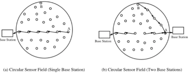
Consider two different sensor network deployments as shown in Figure 1. In Figure 1(b) sensor node Ais one hop away from its nearest base station when two base stations are deployed. For sensor node B the hop-count from its nearest base station is same in both the cases. Thus, by employing two base stations instead of one we have effectively either reduced or retained the hop count of each sensor node in the network. Since the energy consumed in routing a message from any sensor node to its nearest base station is proportional to number of hops the message has to travel, employing multiple base stations effectively reduces the energy consumption per message delivered.
A B
Base Station Base Station
A B
(a) Circular Sensor Field (Single Base Station) (b) Circular Sensor Field (Two Base Stations)
Base Station
Fig. 1. Circular Field of Interest
B. Why move Base Stations?
In [17], the authors demonstrated through experimental results that the sensor nodes which are one-hop away from a base station drain their energy faster than other nodes in the network. The authors attribute this to the fact that nodes which are one hop away from a base station need to forward messages originating from many other nodes, in addition to delivering their own messages. In doing so, these sensor nodes deplete their energy quickly and become inoperational. As a result, many sensor nodes will be unable to communicate with the base stations and the network becomes inoperational.
To increase the lifetime of a sensor network, we propose to employ multiple base stations and periodically change their locations. We propose two strategies to choose base station locations and compare the performance of these strategies with three other strategies. We also propose a routing protocol based on flow information. Through simulations we show that our strategies outperform all the other strategies.
II. SYSTEMMODEL
We make the following assumptions about the network: 1) Each sensor node has a unique pre-configured id. 2) The sensor network is proactive [1] and each node
generates equal amount of data per time unit. We assume that each data unit is of same length.
3) The transmission range of each sensor node is fixed. 4) The transceiver exhibits first order radio model
charac-teristics [17], where energy dissipation for the transmit-ter or receiver circuitry is constant per bit communicated. Also, energy spent in transmitting a bit over a distance
d is proportional to d2. It can also be argued that transmission energy is proportional to d4 [8].
5) There exists a contention free MAC protocol [12] which provides channel access to all the nodes.
6) There exists a multi-hop routing protocol. For example, the Minimum Cost Forwarding (MCF) protocol for large sensor networks [5] can be used.
7) An upper bound on the number of base stations available is fixed and is known a priori.
8) We consider equal periods of time calledrounds. At the beginning of each round new base station locations are computed and stay fixed during that round.
9) Base stations can be located only at certain sites, called feasible sites. Base stations are mounted on unmanned remote controlled vehicles and can be moved from one feasible site to another.
III. PROBLEMFORMULATION
At the beginning of each round, we need to determine the location of the base stations at feasible sites. We refer to this problem as the Base Station Location (BSL) problem.
The sensor network is represented as a graphG(V, E)where (a) V = Vs∪ Vf where Vs represents the sensor nodes
andVf represents the feasible sites.
(b) E⊆V×V represents the set of wireless links1.
Let Kmax be the maximum number of base stations. Let a round consist ofT timeframes. Each sensor node generates one packet of data in every timeframe. At the beginning of a round, let a sensor node i have residual energy REi. A
constraint we impose is that during the round, the total energy spent by sensor node i is at most αREi, where 0 < α ≤ 1
is a parameter. Next, we describe an integer linear program formulation for the BSL problem.
IV. ANINTEGERLINEARPROGRAMFORMULATION
Let yl be a 0-1 integer variable for each l ∈ Vf such
that yl = 1 if a base station is located at feasible site l;
0 otherwise. N(i) = {j : (i, j) ∈ E}. Given G(V, E), α
and Kmax, the following Integer Linear Program (ILP) [9],
[15], denoted byBSLmm(G, α, Kmax), minimizes the
max-imum energy spent, Emax, by a sensor node in a round.
Minimize Emax j∈N(i) xij− k∈N(i) xki = T, i∈V (1) Et j∈N(i) xij+Er k∈N(i) xki ≤ αREi, i∈V (2) l∈Vf yl ≤ Kmax (3) i∈Vs xik ≤ T|Vs|yk, k∈Vf (4) Et j∈N(i) xij+Er k∈N(i) xki ≤ Emax, i∈V (5) xij ≥0, i∈Vs, j∈V; yk ∈ {0,1}, k∈Vf (6)
1Wireless links between sensor nodes and a feasible site refer to the links that would exist if a base station is located at that particular site.
Assuming no data aggregation2, the balance of flow of messages at each node is represented by (1), where xij
represents number of messages node i transmits to j∈ N(i)
in a particular round. LetEr(resp.Et) be the energy spent by
a sensor node in receiving (resp. transmitting) a message.Er
and Et can be calculated from antenna characteristics. Then
the total energy spent by all the nodes during a particular round is bound by (2). The number of feasible sites selected to locate the base stations is limited to at mostKmaxby (3). Constraints
(4) ensure that transmission of messages to a feasible site is possible only if a base station exists at that site. The objective function and constraint set (5) minimize the maximum energy spent by any sensor node during the round.
Another reasonable objective is to minimize total en-ergy consumption during a round. To optimize this objec-tive function we remove the constraint set (5) and change the objective function to MinimizeEti∈Vs
j∈N(i)xij+
Eri∈Vs
k∈N(i)xki. We refer to this problem as
BSLme(G,
α,Kmax). Solving any of these ILPs would give
us the locations of base stations and flow of messages in the network. Since solving integer linear programs can be time consuming, good feasible solutions are sufficient. Next, we describe how the flow information (values ofxij) can be used
to route messages to the selected base stations. V. FLOWBASEDROUTINGPROTOCOL
Sensor nodes can use the flow information obtained by solving the integer linear program to route messages in an energy efficient manner. Consider sensor node A with its incoming and outgoing number of messages as shown in Figure 2. Once a sensor node has this information it would perform its routing as described below.
500.5 n m l k j i 100 200 449.5 200.3 99.2 750.5 A
Fig. 2. Flow Based Routing
(i) For every outgoing link a counter is maintained. The value of the counter is set to the floor of the flow going out on that particular link.
(ii) Whenever a node needs to transmit its packets, it would select one of the outgoing links in a round robin fashion. (iii) If the counter value of the selected link is greater than the number of packets that have to be transmitted, then all the packets are transmitted on that link and counter value is decremented by the number of packets
2Data aggregation refers to the local processing of data carried out at each sensor node. For example, if the goal is to monitor the maximum temperature in a region then it is inefficient to forward all the temperature data to the base station. Instead, each sensor node would transmit only the maximum among the values it has seen so far.
transmitted; otherwise the number of packets equal to the counter value of the link are transmitted along the link and its counter value is set to 0. To transmit the remaining messages outgoing links are selected in a round robin fashion.
(v) If the counter value of all the outgoing links is zero then a link is selected arbitrarily and all the packets are transmitted on this link.
Example: Suppose nodeA in Figure 2 had 250 packets to transmit. If link l was selected then 200 packets would be transmitted on this link and its new counter value would be set to 0. The remaining 50 packets would be transmitted on
mand its counter values would be updated to 450.
The main idea behind this heuristic is that when the number of packets to be transmitted is large, the routes taken by the packets closely follow the flow information on the outgoing links.
VI. IMPLEMENTATIONDETAILS
To implement the proposed solution, we need to address the following issues.
A. Gathering topology information. B. Tracking residual energy of nodes.
C. Updating routing information of all the nodes. D. Solving ILP.
At the beginning of the first round, network topology, required to formulate the ILPs, is not available. In the first round, we propose to select the base station locations randomly and use a modified Minimum Cost Forwarding (MCF) routing protocol3 [5]. Once the network topology is obtained in the first round, it can be used in subsequent rounds to solve the ILPs.
A. Gathering Topology Information
To formulate the ILPs described we need to know the topol-ogy of the sensor network. A contention-free MAC protocol, say SMACS [12], will let each node learn about the identities of its neighbors. Each node then transmits its neighbor list to its nearest base station. The complete sensor network topology can be constructed at one of the base stations.
Apart from the topology information, we need to know which sensor nodes are one-hop away from the feasible sites. We propose to manually deploy one special sensor at each feasible site. The node ids of these special sensors are known a priori. These special sensors participate in the MAC protocol as ordinary sensors. Once the neighbor list of all the nodes is collected at the base stations, sensor nodes one hop away from feasible sites can be determined.
B. Tracking Residual Energy of Nodes
In the beginning, every sensor node has the same amount of energy and this value is known. As routing is deterministic, we know the exact route taken by each message and hence the
3Each sensor node would keep track of all the nodes that are on the shortest path from itself to the base station. When a packet is to be forwarded, the packet is transmitted to only one of these nodes.
energy spent by each node. We can thus compute the residual energy of each node at the end of a round. To account for the possibility of sensor node failure due to environmental reasons we need to either include mechanisms to track source node id of each message or expect each sensor node to transmit a heart beat packet periodically.
C. Updating Routing Information of Each Node
To perform flow-based routing, the sensor nodes need the flow information. We propose to transmit this flow information directly to the sensor nodes from the base station. In doing so, sensor nodes would spend energy only in receiving the messages. In other routing protocols, each node is required to transmit and receive multiple messages to establish routing in-formation [5]. Thus transmitting the flow inin-formation directly to sensor nodes would conserve energy in the sensor network.
D. Solving ILP
Any efficient integer linear programming solver (e.g. CPLEX, Xpress-MP) can be used to solve the BSL problem in each round. As stated earlier, our goal in formulating the integer linear program is not to solve it to optimality but to obtain good feasible solutions in the available time. The integer programs can be solved at one of the base stations.
VII. EVALUATIONMETRICS
The main objective of this study is to increase the useful lifetime of sensor networks. However, a precise definition of the lifetime is application dependent. Some applications might tolerate a loss of considerable number of nodes and still be deemed functional, while in others losing a single sensor node will render the network worthless. Below we discuss some evaluation metrics.
1) Time until the first node dies:This metric indicates the duration for which the sensor network is fully functional. 2) Time until aβ fraction of nodes die:The suitability of this measure is application dependent. Across applica-tions, choosingβ= 0.5seems to be appropriate. Unless specified otherwise, we use this metric to indicate the lifetime of the network.
3) Total number of messages received: Total number of messages received until a β fraction of the nodes die indicates the amount of information collected until that time. This measure is an indicator of the total amount of information collected during its lifetime.
4) Energy spent per round: The total amount of energy spent in routing messages in a round is a short-term measure designed to provide an idea of the energy efficiency of any proposed method in a particular round.
VIII. SIMULATIONRESULTS
To compare the proposed solutions, we simulated a sensor network of 30 nodes randomly distributed in a 30×30 meter-square sensor field. 20 feasible sites were located randomly on the periphery of the sensor field. A maximum of 3 base stations were made available. Each sensor node was provided with an
initial energy of 0.5 J. The transmission range of each sensor node was set to 10 meters. The energy spent in transmitting a bit over a 1 meter distance is taken as 0.1 nJ/bit-m2 [17] and the energy spent in receiving a bit is set to 50 nJ/bit [17]. The packet length is fixed at 200 bits. Each round lasts 100 time-frames. To solve each instance of eitherBSLmm(G,
α,Kmax)
or BSLme(G,
α, Kmax) we used CPLEX (version 7.5) with
a time limit of 4 minutes. The best feasible solution within this time limit was accepted. For each instance, the value of
α was initially set to 0.2 and incremented in steps of 0.2 in case the instance was infeasible.
On this simulated sensor network we implemented follow-ing schemes for a comparative study.
(a) Scheme 1.A single, static base station. (b) Scheme 2.Three static base stations.
(c) Scheme 3. Three mobile base stations with random positioning among the 20 feasible sites.
(d) Scheme 4. Three mobile base stations with locations obtained by solvingBSLme(G,α,Kmax).
(e) Scheme 5. Three mobile base stations with locations obtained by solvingBSLmm(G,α,Kmax).
In the third scheme, at the start of each round base station locations were determined randomly. In schemes 1, 2, 3 and 4 we employed modified MCF routing. Flow-based routing was used in scheme 5.
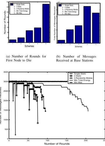
For each of the schemes above, Figure 3(a) compares the time until the first node dies. Scheme 5 significantly outper-forms other schemes. This is not surprising since BSLmm
minimizes the maximum energy spent by a node in a round. Therefore, the outgoing flow from a sensor node is split across various paths (if they exist) leading to the selected base sta-tions. There is an equitable distribution of energy consumption by the sensor nodes in each round. Using flow-based routing, which mimics the network flow obtained byBSLmm, energy dissipation is uniform across all nodes resulting in the network being fully operational for a longer period of time. On the other hand, using BSLme minimizes the total energy usage in a round and does not prevent an individual sensor node from draining more energy than other nodes. As a result, the first node dies relatively quickly when compared to scheme 5. We observed similar trends on networks with 50, 100, 150 and 200 sensor nodes. It can be concluded that irrespective of size of the network, scheme 5 would be the best option available if all the sensor nodes are required to be functional throughout the lifetime of the network.
Figure 3(c) compares the number of messages delivered in each round. Scheme 5 delivers all the messages throughout the lifetime of the network. For all the other schemes, the number of messages delivered decreases with time as the fraction of dead sensor nodes increases. An interesting observation is that with scheme 5, death of the first node (which is a node one-hop away from a base station) is soon followed by the death of all one-hop away nodes and the network becomes inoperational. This will explain the fact that the total number of messages delivered by scheme 5 is less than that of scheme 4 (as shown in Figure 3(b)) 1 2 3 4 5 0 20 40 60 80 100 120 140 160 Number of Rounds Schemes 1 − Single Static 2 − 3 Static 3 − 3 Randomly Mobile 4 − Min Total Energy 5 − Min Max
(a) Number of Rounds for First Node to Die
1 2 3 4 5 0 1 2 3 4 5 6x 10 5
Total Number of Messages Received
Schemes
1 − Single Static 2 − 3 Static 3 − 3 Randomly Mobile 4 − Min Total Energy 5 − Min Max
(b) Number of Messages Received at Base Stations
0 50 100 150 200 250 0 500 1000 1500 2000 2500 3000 3500 Number of Rounds
Number of Messages Received
Single Static 3 Static 3 Randomly Mobile Min Total Energy Min Max
(c) Number of Messages Received at Base Stations in Each Round Fig. 3. Simulation Results
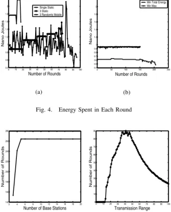
Figures 4(a) and 4(b) compare the energy spent in each round. As expected, scheme 4, in whichBSLme(G, α, Kmax)
minimizes the total energy spent in a round, is the most energy efficient scheme. When base stations are located randomly (scheme 3), the energy consumption varies widely across rounds depending on whether or not the base station locations constitute a good solution. The energy consumption plot in scheme 2 is similar to a step function. In this scheme, whenever a sensor node dies, some shortest path routes are erased and the energy consumption increases and stays the same until a new set of shortest path routes are found.
A. Impact of the Number of Available Base Stations
We assess the impact of the number of base stations on the lifetime of the sensor network by increasingKmax from 1 to
20. We use scheme 5 to determine the base station locations and message routing. As seen in Figure 5(a) increasing the number of base stations beyond a certain threshold value does not affect the lifetime. We offer the following explanation: the lifetime of the network increases with the number of base stations until every sensor node one hop away from a feasible site is one hop away from some base station. Increasing the
0 10 20 30 40 50 60 70 80 90 100 0.4 0.6 0.8 1 1.2 1.4 1.6 1.8 2 2.2x 10 8 Number of Rounds Nano Joules Single Static 3 Static 3 Randomly Mobile (a) 0 50 100 150 200 250 0.4 0.5 0.6 0.7 0.8 0.9 1 1.2 1.4 1.6 1.8 2 2.2x 10 8 Number of Rounds Nano Joules
Min Total Energy Min Max
(b) Fig. 4. Energy Spent in Each Round
2 4 6 8 10 12 14 16 18 20 140 160 180 200 220 240 260 280
Number of Base Stations
Number of Rounds
(a) Number of Base Stations
0 10 20 30 40 50 60 70 80 90 100 0 10 20 30 40 50 60 70 80 90 Transmission Range Number of Rounds (b) Transmission Range
Fig. 5. Parameters Effecting Network Lifetime
number of base stations any further has no advantage and hence does not affect the network lifetime.
B. Impact of Transmission Range
Increasing the transmission range of the sensor nodes changes the topology of the sensor network since the number of one-hop neighbors for a sensor node increases [13]. To study the impact of the transmission range on network life-time, we simulated a sensor network consisting of 100 nodes randomly distributed in a 100 x 100 field with 3 base stations. Scheme 5 was used to determine the base station locations and message routing. Hundred experiments, where experiment
i, i = 1, ...,100 used a transmission range of i meters for
each sensor node, were performed. Figure 5(b) shows a plot of the results. For a very small transmission range (less than 13 meters), there is little or no transmission as for most sensors there is no route to any feasible site. Beyond this point, as the transmission range increases, the connectivity of network increases resulting in an increase in network lifetime. The lifetime reaches a maximum when the transmission range is around 45 meters. A further increase in the transmission range has little impact on the connectivity and the quadratic rate of increase in energy consumption becomes dominant resulting in a quadratic rate of decrease in the network lifetime. We repeated the experiments with energy of each sensor node set to 20 J. The energy spent in transmitting a message was
assumed to be proportional tod4. Similar results were obtained and the maximum lifetime was noticed when the transmission range is 14 meters.
IX. CONCLUSIONS
In this paper we have proposed an energy efficient usage of multiple, mobile base stations to increase the lifetime of wireless sensor networks. Our approach uses an integer linear program to determine the locations of the base stations and a flow-based routing protocol. We conclude that using a rigorous approach to optimize energy utilization leads to a significant increase in network lifetime. Moreover, the tradeoff between solution quality and computing time allows us to compute near-optimal solutions within a reasonable time for the network sizes considered.
To adopt the approach presented in this paper to very large sensor fields, it might be appropriate to decompose the un-derlying flow network into sub-networks and optimize energy usage in each sub-network independently. A challenging and promising direction for future work is to explore the use of graph partitioning algorithms [4], particularly those for finding balanced partitions [6], [11], within such a framework.
REFERENCES
[1] A. Manjeshwar and D.P. Agrawal. TEEN: a routing protocol for enhanced efficiency in wireless sensor networks. Intl. Proc. of 15th Parallel and Distributed Processing Symp., pages 2009 – 2015, 2001. [2] C. M. Okino and M.G. Corr. Statistically Accurate Sensor Networking.
Wireless Communications and Networking Conference, 2002. [3] C. Schurgers and M.B. Srivastava. Energy Efficient Routing in Wireless
Sensor Networks. Military Communications Conference, 2001. [4] D.B. Shmoys. Cut problems and their application to divide-and-conquer.
Approximation Algorithms for NP-hard Problems, PWS Publishing Com-pany, Boston, pages 192 –235, 1997.
[5] F. Ye, A. Chen, S. Liu and L. Zhang. A scalable solution to minimum cost forwarding in large sensor networks.Proc. of Tenth Intl. Conference on Computer Communications and Networks, pages 304 –309, 2001. [6] G. Even, J. Naor, S. Rao, and B. Schieber. Fast approximate graph
partitioning algorithms. Proc. 8th Ann. ACM-SIAM Symp. on Discrete Algorithms, ACM-SIAM, pages 639 – 648, 1997.
[7] G.J. Pottie. Wireless sensor networks. Information Theory Workshop, pages 139 – 140, 1998.
[8] G.J. Pottie and W.J. Kaiser. Wireless integrated network sensors. Communications of the ACM, 43(5):51 – 58, 2000.
[9] G.L. Nemhauser and L.A. Wolsey. Integer Programming and Combina-torial Optimization.Wiley, 1988.
[10] J. Agre and L. Clare. An integrated architecture for cooperative sensing networks.Computer, 33(5):106 – 108, 2000.
[11] J. Chlebikova. Approximability of the Maximally balanced connected partition problem in graphs.Inform. Process. Lett., 60:225 – 230, 1996. [12] K. Sohrabi, J. Gao, V. Ailawadhi and G.J. Pottie. Protocols for self-organization of a wireless sensor network.IEEE Personal Communica-tions, 7(5):16 – 27, 2000.
[13] M.A. Youssef, M.F. Younis and K.A. Arisha. A Constrained Shortest-Path Energy-Aware Routing Algorithm for Wireless Sensor Networks. Wireless Commun. and Networking Conference, 2002, 2:794 –799, 2002. [14] R. Min, M. Bhardwaj, Seong-Hwan Cho, E. Shih, A. Sinha, A. Wang and A. Chandrakasan. Low-power wireless sensor networks.Fourteenth International Conference on VLSI Design, pages 205 – 210, 2001. [15] R.K. Ahuja, T.L. Magnanti, and J.B. Orlin. Network Flows. Prentice
Hall, New Jersey, 1993.
[16] S. Lindsey and C. Raghavendra. PEGASIS: Power-Efficient Gathering in Sensor Information Systems. Intl. Conf. on Communications, 2001. [17] W.R. Heinzelman, A. Chandrakasan and H. Balakrishnan.
Energy-efficient communication protocol for wireless micro sensor networks. Proceedings of the 33rd Annual Hawaii International Conference on System Sciences, pages 3005 – 301, 2000.