Multivariate Ordered Regression
February 28, 2012
Valentino Dardanoni, Antonio Forcina, Paolo Li Donni ABSTRACT
TO BE WRITTEN JEL codes:
Keywords:
1
Introduction
Many interesting problems in economics involve the study of how an ordered response variable depends on a set of regressors. In many situations we may be concerned with the more general problem of modeling how the joint distribution ofseveral closely related ordered response variables (Y1, . . . , YK) depend on a vector of covariatesz. Problems of this kind arise, for example, when we consider different choices made by each subject at a given point in time, or repeated choices on the same item made by each subject at different points in time.1 In the microeconometric literature, the current approach to modelling the joint conditional distribution of ordinal response variables relies on assuming the existence ofK latent variables which form a regression system
Yk∗=z0kτk+k, k= 1, . . . , K
where zk denotes the subset of regressors z relevant to the kth equation; a set of threshold parame-terstransform the continuous latent distribution into the actual discrete one. In addition, the joint distribution for the errorsH(1, . . . , K) may also be specified.
An alternative approach is to consider the conditional distribution of the ordered response variables as a multi-way table of joint probabilities, to arrange these into the vectorπ(z) and to define a suitable multivariate transformation ofπ(z), known aslink function, which makes the dependence on covariates linear
π(z) =g[λ(z)] =g(α+Zβ); (1)
hereZ is a matrix of known constants which depends onzand the vector of parametersλ(z) describe relevant aspects of (Y1, . . . , YK |z) which have, hopefully, interpretation in terms of economic theory. Models of this kind have, essentially, two components:
1If data involve observations taken at different points in time, the model described in this paper can be seen as a
static panel model with free correlations across periods. With panel data, more specific approaches have been designed to take into account individual heterogeneity, lagged dependent variables and serial correlation.
The regression model λ(z) =α+Zβ: This is the parametric component of the model.
The link function π(z) = g[λ(z)]: This is the potentially non parametric component of the model. It maps the linear function of covariatesλ(z) onto a discrete joint distribution.
Equation (1) defines a wide class of multivariate ordered regression models, whose elements are char-acterized by the specific link functiong. Well known examples are thelog-linear and the probitlinks. The log-linear link function (see e.g. Amemiya ([3], Chapter 9) or Agresti ([1], Chapter 4), in spite of its appealing simplicity, does not allow to model the univariate marginals directly, cannot take into account the ordered nature of the response variables, and does not have a latent variable interpreta-tion. On the other hand, the so called multivariate ordered probit model, which is based on the probit link, does not suffer from any of these limitations. However, because of its simplicity, the probit link imposes some strong restrictions to the association structure of the response variables, namely (i) each bivariate marginal distribution has only one association parameter; and (ii) alllog-linear interactions of order higher than two are constrained to zero. In addition, the process of fitting models based on the probit link may be computationally demanding when there are several response variables.
Within the class of model defined by equation (1), we are typically interested in link functions whose elements have, possibly, the following desirable features:
• they describe relevant aspects of (Y1, . . . , YK)|z which have a substantial economic interpreta-tion;
• they take into account the ordered nature of the response variables;
• they make it possible to model the univariate marginals and the association structure directly;
• they have an interpretation in terms of the system of latent equations.
By exploiting recent advances in the theory ofmarginal modelling (Bartolucci, Colombi and Forcina, [4]), we propose a link function having most of the desirable properties listed above. The available theory of marginal models can handle a link function where the association structure is unrestricted, however this would make the exposition heavier with little practical advantages. Though the link function we discuss in this paper implies certain mild constraints on the association structure, it may be further simplified by testable restrictions. In this formulation, the table π(z) which arrays the joint probabilties of the response variables (Y1, . . . , YK) | z is decomposed into two main sets of parameters of interest, namely theglobal logits, which model the marginal distribution of ordered discrete variables, and the global log-odds ratios, which describe their association. As we show in section 2.4 below, these parameters have a natural interpretation in terms of stochastic dominance, thus allowing a clear economic intepretation of estimated parameters.
In Section 2 we derive the main properties of the marginal modeling approach and its relation with the latent variable model. Section 3 discusses the computational properties of maximum likelihood estimates, and the asymptotic distribution of the likelihood ratio under suitable equality and inequality constraints. Section 4 clarifies the use of these models with an application to testing for asymmetric information in the Medigap insurance market.
2
Ordered regression
In order to help the understanding of our approach to the multivariate case, we start by briefly reviewing the well known univariate case with a single ordinal response variable Y, taking value in
{1, . . . , m}. Letq(z) be them−1×1 vector denoting the survival function of Y, conditionally onz: q(z) = (P r(Y >1|z) . . . P r(Y > m−1|z) )0
and notice that the termP r(Y >0|z) = 1 can be omitted. A generalizedordered regression modelis an equation that relatesq(z) toz through a vector valued functiong :<m−1 →(0,1)m−1, known as
alink function(McCullagh and Nelder [12]) which is assumed to be invertible and twice differentiable and such that
q(z) =g(α+Zβ) (2)
whereZ is a matrix of known constants which depend on z.
Since the link function is invertible, there is a well defined set of m−1 parameters which are linearly related toZ:
λ(z) =g−1(q(z)) =α+Zβ. (3) It is well known (see, for example Wooldridge [19], p. 457) that, under a few additional assumptions, the ordered regression model (2) is equivalent to assume the existence of a continuous latent variable Y∗ which follows a linear regression model
Y∗ =τ0+z 0
τ+ (4)
where the erroris independent ofz and has cumulative distribution functionP(≤v) = G(v), and there is a vector ofm−1 unknown parametersγ (called thresholds), withγ1<· · ·< γm−1, such that
Y ≤j ⇔Y∗ ≤γj. Notice that, since we can add an arbitrary constant toτ0 and subtract the same
constant from γ without affecting α, these two parameters cannot be identified simultaneously; in the sequel we assume that τ0 = 0 so that the regression model in (4) has no intercept. When has
a standard logistic distribution, the latent regression model (4) is equivalent to an ordered regression model where P r( ≤ v) = G(v) = ev/(1 +ev). By inverting the survival function P r(Y > j) = G(−γj+z
0
β), it follows that λ(z) is a vector of so-calledglobal logitswhich are linearly related toz λj(z) = log[P r(Y > j|z)/P r(Y ≤j |z)] = (−γj) +z
0
β, j = 1, . . . , m−1, (5) and can be seen as the natural generalization of the standard binary logits when the variable is ordered. In fact, global logits can be interpreted as binary logits computed after dichotomizing the response categories at each cut point into a ‘low’ and a ‘high’ level.
The standardordered logitmodel can be seen as a special case of the ordered regression model (2) withGbeing the logit link. Different choices of the link functionGgive raise to different assumptions on the distribution of the latent regression error and the definition of the parameter vector λ(z). The best known alternative to the ordered logit model is of course the ordered probit model, where Gis the standardized normal cdf.
2.1 Multivariate ordered regression
The univariate latent regression model (4) may be extended to the multivariate case by assuming, in addition the existence ofK latent continuous variables Yk∗, k = 1, . . . , K, such that
Yk∗=z0kτk+k, k= 1, . . . , K, (6) the existence of a joint distribution for the errors 1, . . . , K. It then becomes a seemingly unrelated regression system formulated in terms of latent variables.
LetH denote the joint distribution of the errors so thatH(a1, . . . , aK) =P(1 ≤a1, . . . , K≤aK), and let Hk, k = 1, . . . , K denote the corresponding univariate marginal distributions. The simplest modelling strategy would be to assume that theK error components in the latent regression models are independent, so that the regression system (6) implies K separate ordered regression models of the form
Hk−1[P(Yk > j(k)|z)] =−γj(k)+z 0
kτk, (k= 1, . . . , K, j = 1,· · ·, mk−1) which may be estimated as in the univariate case and no additional theory is required.
However, there are several reasons for modelling also the association structure of (1, . . . , K). Apart from the fact that, by assuming that (1, . . . , K) are independent, we are likely to mispecify
the true model with a loss of efficiency, the main reason for estimating the whole system of latent equations is that the nature and the degree of association between the response variables (conditionally on the covariates) may be of substantive interest, as in the application considered in this paper.
2.2 Multivariate Link Functions as copulas
The probabilities which define the joint density of Y1, . . . , YK conditionally on z, can be displayed in a table with t= QK
1 mk cells. It is convenient to arrange these probabilities into the vector π(z) in lexicographic order by letting variablesYkwith a larger indexkrun faster from 1 tomk; if unrestricted, π(z) belongs to thet-dimensional simplex Π defined by1t0π(z) = 1 andπ(z)≥0.
As in the univariate case, we are interested in invertible and differentiable mappings which allow to link individual response probabilities to a common vector of parameters
π(z) =g[λ(z)] =g(α+Zβ) =g(Xψ), (7) where the elements ofZ are known functions of the vector of covariatesz,X equals to (I Z), and ψ= (α0 β0)0 collects the model parameters. In view of the fact that the marginal logits are directly related to the univariate latent regression models, it may be convenient to partition λ(z) into two components. The first one, denoted by λu(z), contains the s = PK
k=1(mk−1) global logits which determine the univariate marginal distributions, while the second one, denoted by λa(z), contains a suitable subset of the remaining t−1−s parameters which model the association between the K response variables. Thus, it is convenient to rewrite the regression system (7) above as
λ(z) = λ u(z) λa(z) ! = α u+Zuβu αa+Zaβa ! =Xψ, (8)
whereαu,βu and Zu denote respectively the intercepts, the regression coefficients and the covariate matrix for the set of univariate logits, whileαa,βaandZarefer to those for the association parameters. By modelling the univariate component directly, the association component of the link function outlined above defines a multivariate copula, a conceptual tool for modeling the association among the errors in the K regression equations in a way which treats the response variables in a symmet-ric fashion. Sklar’s Theorem implies that any continuous distribution F may be determined by its marginal distributions Fk and a copula CF(u1, . . . , uK) = F(F1−1(u1), . . . , FK−1(uK)), uk ∈ [0,1] for all k; thus a copula describes the association structure of F irrespective of its univariate marginals. Nelsen [14] provides an excellent introduction to copulas and their properties. This tool is particularly appropriate for describing the association between ordinal variables because copulas are invariant to strictly monotone transformations of the random variables; the other basic property of copulas is that univariate marginals and association structure may be modelled separately and then combined. Therefore, the latent regression model (6) above can be described by the set of regression coefficients βk, the threshold parameters γk, the univariate marginal distribution of the k and the copula CH which in turn may also depend on covariates.
A well known family of parametric copulas is the Gaussian copula: Cρ(u1, . . . , uK) = ΨK(Ψ−11(u1), . . . ,Ψ−11(uK),ρ)
where ΨQ denotes the standard Q-variate normal distribution and ρ is the K(K−1)/2 vector of all bivariate correlation coefficients. When the Gaussian copula is combined with K standard normal marginal distributions it gives the multivariate normal distribution, which, when employed in the latent regression model (6) gives rise to the multivariate ordered probit model (sometimes also called themultiresponse ordered probit model).
Though this model may look appealing, the set of discrete multivariate distributions which are compatible with this copula is very limited. The reason is that, once the cut points are determined in accordance with the univariate marginals, each discrete bivariate marginal distribution, say (Yk, Yh), has (mk−1)(mh−1) additional free cells which are not constrained by the univariate marginals. Under the Gaussian copula all of these probabilities must conform to a bivariate normal and are determined by a single additional parameter (the correlation coefficient). This implies a rather strong restriction unless, of course, the underlying response variables are binary.
2.3 The Multivariate Ordered Logit Model
The copula that we are going to describe in this section is determined by a suitable set of interaction parameters which, together with the global logits (of which they are the natural extension), constitute a parametrization of a relevant subset of Π which is of more direct interest. The approach that can be derived from this formulation has two main advantages with respect to the Gaussian copula:
1. the parameterization is easily invertible without the need for numerical integration;
2. the dependence structure is more flexible because, in the unrestricted model, the number of parameters that determine each bivariate distribution equals the number of free cells in the corresponding frequency table.
However, when the association parameters are constrained to be equal, the complexity of our model is identical to that of the Gaussian copula.
2.3.1 Global interaction parameters
Dale (1986) was among the first to consider this parametrization in the bivariate case; an extension to multivariate distributions see Molenberghs and Lesaffre [13]; Bartolucci, Colombi and Forcina [4] provided a general framework for parameterizing discrete distribution with different kind of marginal interaction parameters; some of their results are used here. Loosely speaking, an interaction term is a parameter measuring the association among a set of variables, say I ⊆ (1, . . . , K), which may be defined within a marginal distribution, sayM, such thatI ⊆ M. In the following we restrict atten-tion to bivariate interacatten-tions defined within the corresponding bivariate distribuatten-tion. The bivariate interactions, which are the key association parameters in our model, are called global log-odds ratios, and, for any two response variables Yi and Yj, dichotomized at the cut point ci and cj respectively, may be written as
λ{i j}(ci, cj |z) = log (
P r(Yi > ci, Yj > cj |z)P r(Yi ≤ci, Yj ≤cj |z) P r(Yi ≤ci, Yj > cj |z)P r(Yi > ci, Yj ≤cj |z) )
2.3.2 The link function and its inverse
Recall that the multinomial distribution, being a member of the exponential family, may be also pa-rameterized by a vector, say θ(z), of canonical parameters; these are log-linear parameters defined within the overall joint distribution (rather than the corresponding marginals). Though these param-eters do not have, usually, a direct interpretation, they can be easily converted into probabilities and provide a useful tool for defining the link function and its inverse.
The link function that we propose is such that each univariate distributionYiis determined bymi− 1 global logits, each bivariate distributionYi, Yj is determined by (mi−1)(mj−1) global interactions and all log-linear interactions of order greater than two are constrained to 0. LetΠDdenote the subset
of the probability simplex satisfying the above restrictions andv=P
i(mi−1) +Pi>j(mi−1)(mj−1). Bartolucci, Colombi and Forcina [4] provide a simple algorithm for constructing a design matrixGD
such that, whenθ(z) varies in <v,
π(z) = exp[GDθ(z)] 10exp[GDθ(z)]
varies in ΠD; ([4], Appendix) provide an algorithm for constructing a contrast matrix C and a
marginalization matrixM such that
λ(z) = λ u(z) λa(z)
!
=Clog[M π(z)], ∀π(z)∈ΠD (9)
LetL={λ(z) :λ(z) =Clog[M π(z)] for someπ(z)∈ΠD}denote the space of compatible marginal
interaction parameters. We can now state the main result of this section:
Theorem 1 The mapping defined by (9) fromΠD toLis invertible and differentiable and thus defines
The theorem is a special case of Theorem 1 in Bartolucci, Colombi and Forcina[4] who consider a more general class of hierarchical parametrization withI ⊆ M.
Unfortunately (9) has no analytical inverse; however a numerical inverse may be computed by a Newton algorithm and is extremely fast and reliable.
Lemma 1 The mapping from λ(z) to θ(z) ∈ <v, or equivalently π(z) ∈ Π
D, may be computed by
the following algorithm:
1. at the initial step choose a value θ(0) such that λ(0) is sufficiently close to λ(z);
2. at theh-th step update the vector of canonical parameters by the first order approximation θ(h)=θ(h−1)+D[λ(z)−λ(h−1)]
where D =∂θ/∂λ0 =[Cdiag(M π)−1Mdiag(π)GD]−1
3. iterate until the norm ofλ(z)−λ(h−1) is close to 0.
The Lemma is a direct application of the Newton algorithm. Since the mapping fromθ(z) toλ(z) has continuous second order derivatives ∀θ(z) whose elements are finite, the result may be derived, for example, from Theorem 4.4 in S¨uli and Mayers [18].2 Forcina and Dardanoni [9] study in detail the nature of the copula defined by the multivariate ordered logit link function and show that there exists a continuous multivariate latent distribution which has exactly the same parameters as its discrete analog.
2.4 Interpretation of the parameters in terms of stochastic dominance
The main parameters of interest in our model are the univariate global logits and the bivariate global log-odds ratios. To understand their economic significance in this section we explore their properties in terms of stochastic dominance.
2.4.1 Global logits
It is interesting to note that the global logits satisfy a stochastic ordering property which seems particularly appropriate when the response variables have an ordinal nature, in the sense that their relevant properties are preserved under arbitrary monotonic transformations:
Lemma 2 Given two discrete ordered random variables Yh and Yk in {1,· · ·, m}, the following con-ditions are equivalent:
1. E[u(Yh)|z]≥E[u(Yk)|z]for any function u which is non decreasing; 2. Yh is stochastically greater than Yk conditionally on z;
3. log[P(Yh > j|z)/P(Yh ≤j|z)]≥log[P(Yk> j |z)/P(Yk≤j |z)]∀j < m.
2In our experience, by settingθ(0) = 0
v, the algorithm always converges as long as λ(z) is not too close to the
boundary of the parameter space; this may happen for example when one or more elements are much larger than 20 in modulus.
Proof The equivalence between the first two conditions is well known (see for example Hadar and Russell [10] Theorems 1 and 2). The equivalence with the third condition follows by noting that global logits are strictly increasing transformations of the cumulative distribution.
If we regress a global logit on a given covariate and the regression coefficient is positive, then the response variable becomes stochastically larger whenever that covariate increases; because of this, regression coefficients in the ordered logit regression have a direct interpretation in terms of stochastic dominance.3
2.4.2 Global log-odds ratios
The log-odds ratios, which determine the association for any pair of responses, are also closely related to the notion of positive quadrant dependence (P QD), an instance of positive dependence between ordinal variables first introduced by Lehmann [11]: two random variables Yh, Yk taking values in
{1,· · ·, mh} and{1,· · ·, mk} areP QD if
P r(Yh ≤i, Yk ≤j)≥P r(Yh ≤i)P r(Yk≤j),∀ i∈ {1,· · ·, mh}, j ∈ {1,· · ·, mk},
which intuitively means that, compared to the case of independence, ”small” values ofYh tend to go with ”small” values ofYk. Negative quadrant dependence is defined by reversing the inequality above. The ordinal nature ofYh and Yk seems to motivate the requirement that their relevant properties should be preserved under arbitrary monotonic transformations. The following result in the theory of stochastic orderings links the notion of positive dependence,P QD, to the log-odds ratios:
Lemma 3 Given a pair of discrete ordered random variablesYh andYk taking values in {1,· · ·, mh} and {1,· · ·, mk}, and any pair of increasing functions u, v, the following conditions are equivalent:
1. Cov[u(Yh), v(Yk)|z]≥0;
2. Yh and Yk are P QD conditionally on z;
3. the set of log-odds ratios λh,k(ci, cj |z)≥0 for all ci < mh, cj < mk. ProofSee Nelsen [14], exercises 5.22 and 5.27, p. 153-4.
This result may be interpreted as saying that, if the ordered variables are the discrete version of continuous latent variables discretized at arbitrary thresholds, the log-odds ratios are the most appropriate measure of association, in the sense that the sign of the dependence between the underlying variables is preserved, irrespective of how the ordered categories are constructed.
3
Statistical inference
3.1 Hypotheses of interestA convenient feature of the multivariate ordered regression model defined by equation (8) is that
all the relevant hypotheses of interest can be expressed in the form of linear equality and inequality
3Notice instead that the standard interpretation of ordered logit coefficients (see for example Crawford, Pollak and
Vella, 1998), which refers to the density rather than the cumulative distribution of the response variable, implies often a rather convoluted interpretation.
constraints on the vector of model parametersψ = (α0 β0)0. Arelevant set of testable restrictions consists in assuming that the bivariate association parameters do not depend on the cut points, an as-sumption which is the multivariate analog of thePlackett distribution. The family of bivariate Plackett distributions, introduced by Plackett [15], has been extended to the multivariate case by Molenberg and Lesaffre [13]. Forcina and Dardanoni [9] discuss the multivariate ordered regression model under the Plackett distribution; that model is a close analog to the multivariate ordered probit model, with the correlation coefficients replaced by the corresponding bivariate log-odds ratios. The advantage of our modeling strategy is that these assumptions are imposed by means of testable restrictions.
Linear inequality constraints may be used to test a stochastic dominance effect of certain covariates on a set of latent regressions. We could also be interested to test positive dependence between a pair of responses against conditional independence by imposing that all the (mh−1)(mk−1) log-odds ratios are positive against being zero. Generally speaking, any set of hypothesis of interest may be expressed in the form
H:{ψ :Eψ=0, U ψ ≥0}
by an appropriate choice of the ”equality” and ”inequality” matricesE and U. Clearly, the case with E or U equal to the null matrix correspond to restriction with only inequalities or only equalities respectively.
3.2 Likelihood inference
Suppose we have independent observations (Y1i, . . . , YKi,zi) for a sample of n units. Let t(zi) be a vector of size Q
mk made of 0’s except for the element corresponding to the observed combination of (Y1, . . . , YK) for the ith unit which is equal to 1. To simplify notations, in the sequel we write t(i) instead oft(zi); a similar convention will be adopted for any vector which depends on zi. Under independent sampling, conditionally onzi,t(i) has a multinomial distribution with vector of probabil-itiesπ(i). In order to manipulate the likelihood function more easily, we write the multinomial as an exponential family with the vector of canonical parameters introduced before Lemma 2; in practice, these are all the log-linear interactions which belong to the hierarchical set of marginals D, so that λ(i) has the same dimension asθ(i).
The contribution of the ith unit to the log likelihood is L(i) =t(i)0log[π(i)]
which, by expressingπ(i) in terms of the canonical parameters, may be written as L(i) =t(i)0GDθ(i)−log[1 0 exp(GDθ(i))]. If we define D(i) = ∂θ(i) ∂λ(i)0 = " ∂λ(i) ∂θ(i)0 #−1 = [Cdiag[M π(i)]−1Mdiag[π(i)]GD]−1
the individual score vector is easily computed by differentiatingL with respect to the vector of model parametersψ by the chain rule
s(i) = ∂L(i) ∂ψ = ∂λ(i)0 ∂ψ ∂θ(i)0 ∂λ(i) ∂L(i) ∂θ(i) =X(i) 0 D(i)0GD 0 [t(i)−π(i)].
The individual contribution to the expected information matrix has also a simple form because E{GD 0 [t(i)−π(i)]}=0 F(i) =−E " ∂2L(i) ∂ψ∂ψ0 # =X(i)0D(i)0GD 0 Ω(i)GDD(i)X(i)
where Ω(i) = diag[π(i))−π(i)π(i)0] is the kernel for the variance matrix of the multinomial distri-butions.
Having assumed that the units are independent, the log-likelihood is L(ψ) = P
iL(i), thus the score vectors(ψ) = ∂L∂ψ(ψ) and the expected information matrixF(ψ) =−E(∂2L(ψ)
∂ψ∂ψ0) can be obtained by summing over units. Dardanoni, Fiorini and Focina (2012), for the case of two ordinal responses, discuss an approach to likelihood inference similar to the one proposed here.
3.3 Parameter estimation
Maximum likelihood estimates of ψ under H can be obtained by an algorithm which extends to inequality constraints the seminal algorithm introduced by Aitchison and Silvey [2]. The Aitchison and Silvey algorithm (see for instance Colombi and Forcina [7]) is based on iterated linear approximations of the regression model onto the space of the canonical parameters which are variation independent; the approximation is updated until convergence. Formally:
• assign a starting valueψ(0) which produces compatible λ(i) for all units;
• at the hth step, compute a linear approximation of θ(i) and a quadratic approximation of the log likelihood θ(i)h = θ(i)h−1+D(i)h−1[X(i)ψh−λ(i)h−1] Qh(ψ) = −(ψ−bh) 0 Fh−1(ψ−bh)/2 wherebh= [Fh−1]−1[sh−1+sh−1 1 ] andsh −1 1 = P iX(i) 0 D(i)h−10G D 0 Ω(i)h−1G DD(i)h−1λ(i)h−1
• setψh to be equal to the constrained maximum ofQh(ψ) underH,
• iterate until convergence, that is, until the estimate of λ is sufficiently stable and the linear approximation ofθ is sufficiently accurate.
The starting point must be chosen so that the correspondingλ(i)0 is compatible for all subjects. This may be achieved by setting to zero the intercepts of association parameters and all the regression coefficients corresponding to the covariates. Notice that, when inequality constraints are present, so thatU is not the null matrix, the maximization ofQh(ψ) at each step requires a quadratic optimiza-tion which is itself iterative; there are many algorithms for quadratic optimizaoptimiza-tion under inequality constraints, which are usually very fast and reliable. Since the likelihood function and the transforma-tion fromθ(i) toλ(i) satisfy the conditions discussed by Aitchison and Silvey ([2] p. 817), it follows that, asnincreases, the probability that a constrained maximum exists tends to one. If the algorithm converges, it must converge to a local maximum by the argument of Aitchison and Silvey ([2] p. 826). Notice that our parameterization satisfies the two basic assumptions given by Rao ([16], p.296), namely identifiability and continuity of the transformation fromψtoπ. It follows that, provided that
ψ0, the true value ofψ underH, is an interior point of the parameter space, them.l.e.ofψ under H
exists, is consistent and has an asymptotic normal distribution.
4
An application to the Positive Correlation Test of asymmetric
information in insurance markets
There is a constantly growing body of empirical literature studying the existence of asymmetric in-formation in insurance markets (for a review see Cohen and Spiegelman [6] and Einav et al. [8])). Standard economic theory predicts that risk occurrence and insurance coverage are positively corre-lated, since individuals who know to be riskier tend to buy more coverage (adverse selection) or to consume more for a given structure of the contract (moral hazard). The theoretically predicted pos-itive correlation has inspired the seminal “Pospos-itive Correlation” (PC) test by Chiappori and Salani´e [5]. The PC test rejects the null of absence of asymmetric information in a given insurance market when, conditional on consumers’ characteristics used by insurance companies to price contracts, in-dividuals with more coverage experience more of the insured risk. In their seminal paper Chiappori and Salani´e [5] provide simple empirical strategies to test the positive correlation hypothesis when both insurance coverage and risk occurrence are binary variables. The PC test has been applied to hundreds of various insurance markets, including acute health, long-term care, automobile, annuities, life, reverse mortgages and crop. In most applications, its implementation relies on a simple bivariate probit model, where the null of the absence of private information is tested by absence of residual errors correlation.
In this application, we explain how our approach can be used to empirically implement the PC test when insurance coverage and risk are ordered categorical. We focus on the Medigap health insurance market in the US. Medigap is a private health insurance designed to cover some “gaps” in the coverage left by Medicare, which is a public health insurance program which provides coverage for all individuals aged 65 in US. In general the structure of Medicare is such that it leaves beneficiaries at risk for large out-of-pocket expenses. As a result, elderly may purchase voluntary supplemental private policies, such as Medigap, to fill Medicare’s gaps in non-covered health care services and limit cost sharing. Medigap insurance market is highly regulated by Federal law, which designed a particular mechanism favoring the insured. In particular, insurance companies must offer a basic plan if they offer any other more generous plan; in addition, there is an enrolment period where insurance companies cannot refuse any insurer even if there are pre-existing conditions. Finally, federal regulation allows insurance company to set premium by individual’s age and gender.
To study the Medigap health insurance market we use data from the Health and Retirement Study conducted during the year 2002.4 Since we focus specifically on Medigap, we exclude those individuals younger than 65 and that received additional coverage through a former employer, spouse or are covered by some other government agency. We then consider only those who bought deliberately additional coverage. The final sample size is then given byN = 3290 observations. Since the Medigap plans differ on how generous is the coverage, we define the Medigap insurance coverage indicator (Plan) equals 0 if the individual has no coverage, 1 if she is covered by Medigap plan A or B, and 2 if
she is covered by any other more generous Medigap plan. Risk occurrence is measured by the number of doctor visits and hospital admissions in the previous two years. Since only a very small number of elders had no doctor visits, we constructed the variableDoc, which takes 0 if individual had less than five doctor visits, 1 if she had between five and ten, and 2 if she visited a doctor more than ten times. Since a very small number of elders had more than two hospital admissions, we defined the variable Hosp equals 0 if respondent had no hospital admission, 1 if she had one hospital admission and 2 if she had at least two hospital inpatient staying. Finally, given that Federal Law allows insurance companies to set premium according to the insured’s age and gender, we use as control only whether the individual is a female (Fem) and 26 age dummy variables ranging from 65 to 90 years old or more.
4.1 Empirical strategy and results
Let i = 1, . . . , N denote individual, zi, denote the vector collecting age and gender of individual i, and P lani,Doci, and Hospi denote insurance coverage, and doctor and hospital use of individuali. We can rewrite model (6) as
P lan∗ =αp+z0βp+p Doc∗ =αd+z0βd+d Hosp∗=αh+z0βh+h
(10)
whereαandβare vectors of unknown parameters, and the errorsk,k=p, d, hhave standard logistic marginal distribution but unspecified association structure (copula). Within this structure, the null of the absence of asymmetric information amounts to testing independence of p, d and p, h.
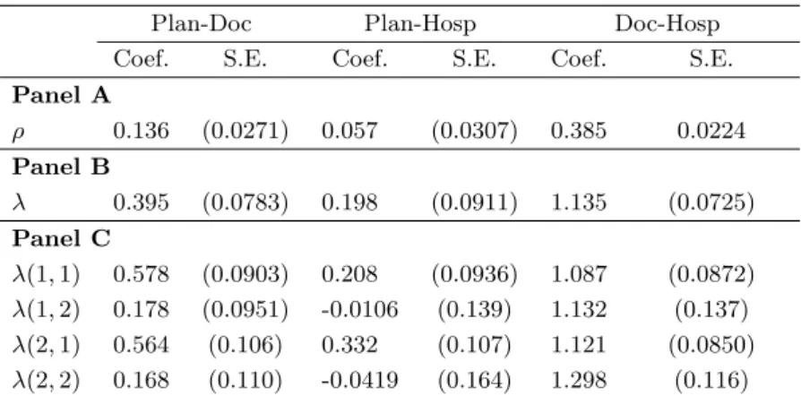
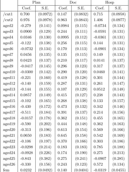
If we assume thatp, d, h in model (10) are jointly distributed as multivariate normal with stan-dard marginal distributions we obtain the multivariate ordered probit which can be estimated by simulated Maximum Likelihood using for example the Stata CMP module (Roodman [17]). Esti-mated coefficients are reported in table 2, and correlation terms are reported in Panel A of table 4. The correlation between P lan and Doc strongly rejects the null of asymmetric information; on the other hand, the null of no asymmetric information between P lanand Hosphas a p-value of 0.065.
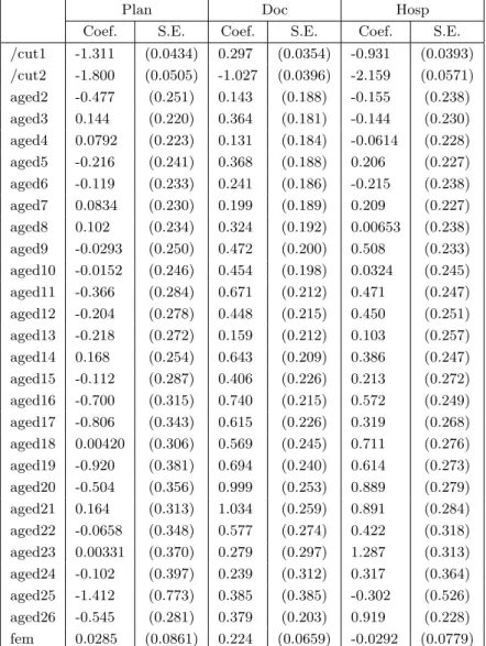
As comparison, table 3 and Panel B of table 4 report estimated coefficients of our multivariate logit model with the Placket restriction, which has the same complexity (same number of parameters) of the multivariate probit since it restricts each bivariate association to one single parameter. A glance of the tables reveals that the two models (probit and Plackett) give a very similar qualitative picture. Allowing for the different scale, the covariates’ parameters follow very similar patterns, and, more importantly, association coefficients (correlation coefficients for the probit and log-odds ratios for the logit) have very similar z-ratios and significance. Thus, the main advantage of our model is that it does not require use of simulated methods for estimation, and tends to be more accurate and faster.5 Both the multivariate probit and the multivariate logit with Plackett restrictions however suffer from the limitation of imposing a restrictive structure to the bivariate associations of interest. To relax the Plackett assumption, we allowλ{p,d},λ{p,h} andλ{d,h} to vary across the categories ofP lan,
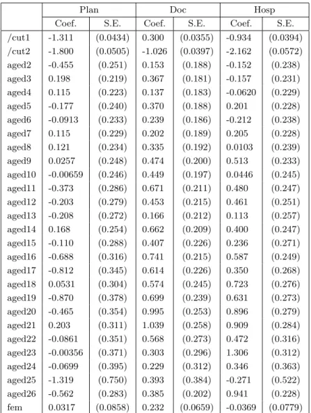
Doc and Hosp. Since these variables have three categories, this implies estimating 2×2×3 = 12 association parameters rather then three with the Palckett restriction. Estimated parameters for this
5
On a 2.4 GHz P8600 processor, estimating the logit model took about 178 seconds, which is about half the time the time (358 seconds) employed estimating the CMP module with the default number of draws set by the program (115)).
model are reported in table 4 and in Panel C of table 1. A glance at Panel C of table 1 reveals that, while the 4 association coefficients for the two health care variables Doc and Hospare similar across categories, they differ in the case of coverage/risk associationP lan−Doc and P lan−Hosp. A formal test of the Plackett assumption λ{p,d}(1,1) = λ{p,d}(1,2) = λ{p,d}(2,1) = λ{p,d}(2,2) and
λ{p,h}(1,1) = λ{p,h}(1,2) = λ{p,h}(2,1) = λ{p,h}(2,2) has LR test statistic equal to 31.90 and is
asymptotically distributed as aχ2 with 12−3 = 9dof. Therefore the null is overwhelmingly rejected with a p-value equal to 0.0002.6
Table 1: Estimated correlation terms
Plan-Doc Plan-Hosp Doc-Hosp
Coef. S.E. Coef. S.E. Coef. S.E.
Panel A ρ 0.136 (0.0271) 0.057 (0.0307) 0.385 0.0224 Panel B λ 0.395 (0.0783) 0.198 (0.0911) 1.135 (0.0725) Panel C λ(1,1) 0.578 (0.0903) 0.208 (0.0936) 1.087 (0.0872) λ(1,2) 0.178 (0.0951) -0.0106 (0.139) 1.132 (0.137) λ(2,1) 0.564 (0.106) 0.332 (0.107) 1.121 (0.0850) λ(2,2) 0.168 (0.110) -0.0419 (0.164) 1.298 (0.116) Notes: For all equations control variables are age and gender dummies. Omitted age category is 65 years old.
Estimated parameters reveal that the coverage/risk correlation is not homogeneous across coverage and risk categories. In particular, association between coverage and risk, for both doctor visits and hospital stays, is significantly positive only for moderate levels of health care use. In other words, conditional on age and gender, the null of no asymmetric information cannot be rejected if actual risk is defined as heavy use of health resources.
Our results show that allowing association to vary across categories may provide a clearer picture of the effect underlying individual’s heterogeneity. Recall, however, that finding residual coverage/risk correlation does not necessarily help to understand whether this is due to the structure of the contract (moral hazard) or rather to the existence of unpriced (by the insurer) individual risk (adverse selection).
References
[1] Agresti, A. (2002). Categorical data analysis. Wiley-Interscience.
[2] Aitchison, J. and Silvey, S. D. (1958). Maximum-likelihood estimation of parameters subject to restraints.The Annals of Mathematical Statistics 29: pp. 813–828.
[3] Amemiya, T. (1985).Advanced econometrics. Harvard University Press.
6For robustness we have also computed the LR test relaxing the equality assumptions separately. The LR test
statistics for the null of equalλs betweenP lan−DocandP lan−Hospare equal to 18.70 and 9.47, which are rejected with ap-value of 0.0003 and 0.0237 respectively. On the contrary the LR test statistics for the null of equalλs between docandhospis equal to 3.7963, which is not rejected with ap-value 0.2843.
[4] Bartolucci, F., Colombi, R. and Forcina, A. (2007). An extended class of marginal link functions for modelling contingency tables by equality and inequality constraints.Statistica Sinica 17: 691. [5] Chiappori, P.-A. and Salani´e, B. (2000). Testing for asymmetric information in insurance markets.
The Journal of Political Economy 108: 56–78.
[6] Cohen, A. and Spiegelman, P. (2010). Testing for adverse selection in insurance markets.Journal of Risk and Insurance 77: 39–84.
[7] Colombi, R. and Forcina, A. (2001). Marginal regression models for the analysis of positive association of ordinal response variables.Biometrika 88: pp. 1007–1019.
[8] Einav, L., Finkelstein, A. and Levin, J. (2010). Beyond testing: Empirical models of insurance markets. Annual Review of Economics 2: 311–336.
[9] Forcina, A. and Dardanoni, V. (2008). Regression models for multivariate ordered responses via the plackett distribution. Journal of Multivariate Analysis 99: 2472–2478.
[10] Hadar, J. and Russell, W. R. (1969). Rules for ordering uncertain prospects. The American Economic Review 59: pp. 25–34.
[11] Lehmann, E. L. (1966). Some concepts of dependence.The Annals of Mathematical Statistics 37: pp. 1137–1153.
[12] McCullagh, P. and Nelder, J. (1989). Generalized linear models (Monographs on statistics and applied probability 37). Chapman Hall, London.
[13] Molenberghs, G. and Lesaffre, E. (1994). Marginal modeling of correlated ordinal data using a multivariate plackett distribution. Journal of the American Statistical Association 89: pp. 633– 644.
[14] Nelsen, R. (2006).An introduction to copulas. Springer Verlag.
[15] Plackett, R. L. (1965). A class of bivariate distributions. Journal of the American Statistical Association 60: pp. 516–522.
[16] Rao, C. (1973).Linear statistical inference and its applications. Wiley (New York).
[17] Roodman, D. (2011). Fitting fully observed recursive mixed-process models with cmp. Stata Journal 11: 159–206(48).
[18] S¨uli, E. and Mayers, D. (2003). An introduction to numerical analysis. Cambridge University Press.
[19] Wooldridge, J. (2002). Econometric analysis of cross section and panel data. The MIT press.
Table 2: Estimatedα and β parameters for the multivariate probit model
Plan Doc Hosp
Coef. S.E. Coef. S.E. Coef. S.E.
/cut1 0.700 (0.0972) 0.147 (0.0832) 0.715 (0.0958) /cut2 0.976 (0.0978) 0.963 (0.0843) 1.406 (0.0977) aged2 -0.279 (0.141) 0.0984 (0.115) -0.0734 (0.134) aged3 0.0900 (0.129) 0.244 (0.111) -0.0591 (0.131) aged4 0.0346 (0.130) 0.0995 (0.112) -0.0361 (0.131) aged5 -0.122 (0.138) 0.256 (0.115) 0.144 (0.131) aged6 -0.0732 (0.134) 0.170 (0.113) -0.0901 (0.134) aged7 0.0456 (0.135) 0.135 (0.115) 0.149 (0.131) aged8 0.0423 (0.137) 0.210 (0.117) 0.0141 (0.137) aged9 -0.0417 (0.145) 0.296 (0.123) 0.317 (0.137) aged10 -0.0300 (0.142) 0.290 (0.120) 0.0460 (0.141) aged11 -0.221 (0.160) 0.419 (0.128) 0.301 (0.144) aged12 -0.140 (0.159) 0.287 (0.131) 0.261 (0.147) aged13 -0.144 (0.155) 0.107 (0.129) 0.0512 (0.148) aged14 0.0857 (0.149) 0.415 (0.127) 0.238 (0.143) aged15 -0.102 (0.165) 0.268 (0.138) 0.133 (0.157) aged16 -0.430 (0.172) 0.473 (0.132) 0.342 (0.146) aged17 -0.511 (0.184) 0.391 (0.137) 0.214 (0.156) aged18 -0.0157 (0.178) 0.362 (0.151) 0.455 (0.165) aged19 -0.590 (0.202) 0.444 (0.148) 0.362 (0.163) aged20 -0.313 (0.196) 0.613 (0.154) 0.569 (0.166) aged21 0.0650 (0.183) 0.645 (0.158) 0.542 (0.169) aged22 -0.106 (0.197) 0.370 (0.166) 0.303 (0.186) aged23 -0.0298 (0.214) 0.183 (0.183) 0.785 (0.188) aged24 -0.0928 (0.226) 0.174 (0.190) 0.275 (0.213) aged25 -0.843 (0.382) 0.275 (0.241) -0.0907 (0.285) aged26 -0.330 (0.156) 0.243 (0.123) 0.572 (0.134) fem 0.0232 (0.0492) 0.140 (0.0404) -0.0319 (0.0455)
Table 3: Estimatedα and β parameters for the Plackett model
Plan Doc Hosp
Coef. S.E. Coef. S.E. Coef. S.E.
/cut1 -1.311 (0.0434) 0.297 (0.0354) -0.931 (0.0393) /cut2 -1.800 (0.0505) -1.027 (0.0396) -2.159 (0.0571) aged2 -0.477 (0.251) 0.143 (0.188) -0.155 (0.238) aged3 0.144 (0.220) 0.364 (0.181) -0.144 (0.230) aged4 0.0792 (0.223) 0.131 (0.184) -0.0614 (0.228) aged5 -0.216 (0.241) 0.368 (0.188) 0.206 (0.227) aged6 -0.119 (0.233) 0.241 (0.186) -0.215 (0.238) aged7 0.0834 (0.230) 0.199 (0.189) 0.209 (0.227) aged8 0.102 (0.234) 0.324 (0.192) 0.00653 (0.238) aged9 -0.0293 (0.250) 0.472 (0.200) 0.508 (0.233) aged10 -0.0152 (0.246) 0.454 (0.198) 0.0324 (0.245) aged11 -0.366 (0.284) 0.671 (0.212) 0.471 (0.247) aged12 -0.204 (0.278) 0.448 (0.215) 0.450 (0.251) aged13 -0.218 (0.272) 0.159 (0.212) 0.103 (0.257) aged14 0.168 (0.254) 0.643 (0.209) 0.386 (0.247) aged15 -0.112 (0.287) 0.406 (0.226) 0.213 (0.272) aged16 -0.700 (0.315) 0.740 (0.215) 0.572 (0.249) aged17 -0.806 (0.343) 0.615 (0.226) 0.319 (0.268) aged18 0.00420 (0.306) 0.569 (0.245) 0.711 (0.276) aged19 -0.920 (0.381) 0.694 (0.240) 0.614 (0.273) aged20 -0.504 (0.356) 0.999 (0.253) 0.889 (0.279) aged21 0.164 (0.313) 1.034 (0.259) 0.891 (0.284) aged22 -0.0658 (0.348) 0.577 (0.274) 0.422 (0.318) aged23 0.00331 (0.370) 0.279 (0.297) 1.287 (0.313) aged24 -0.102 (0.397) 0.239 (0.312) 0.317 (0.364) aged25 -1.412 (0.773) 0.385 (0.385) -0.302 (0.526) aged26 -0.545 (0.281) 0.379 (0.203) 0.919 (0.228) fem 0.0285 (0.0861) 0.224 (0.0659) -0.0292 (0.0779)
Table 4: Estimated α andβ parameters
Plan Doc Hosp
Coef. S.E. Coef. S.E. Coef. S.E.
/cut1 -1.311 (0.0434) 0.300 (0.0355) -0.934 (0.0394) /cut2 -1.800 (0.0505) -1.026 (0.0397) -2.162 (0.0572) aged2 -0.455 (0.251) 0.153 (0.188) -0.152 (0.238) aged3 0.198 (0.219) 0.367 (0.181) -0.157 (0.231) aged4 0.115 (0.223) 0.137 (0.183) -0.0620 (0.229) aged5 -0.177 (0.240) 0.370 (0.188) 0.201 (0.228) aged6 -0.0913 (0.233) 0.239 (0.186) -0.212 (0.238) aged7 0.115 (0.229) 0.202 (0.189) 0.205 (0.228) aged8 0.121 (0.234) 0.335 (0.192) 0.0103 (0.239) aged9 0.0257 (0.248) 0.474 (0.200) 0.513 (0.233) aged10 -0.00659 (0.246) 0.449 (0.197) 0.0446 (0.245) aged11 -0.373 (0.286) 0.671 (0.211) 0.480 (0.247) aged12 -0.203 (0.279) 0.453 (0.215) 0.461 (0.251) aged13 -0.208 (0.272) 0.166 (0.212) 0.113 (0.257) aged14 0.168 (0.254) 0.662 (0.209) 0.400 (0.247) aged15 -0.110 (0.288) 0.407 (0.226) 0.236 (0.271) aged16 -0.688 (0.316) 0.741 (0.215) 0.587 (0.249) aged17 -0.812 (0.345) 0.614 (0.226) 0.350 (0.268) aged18 0.0531 (0.304) 0.574 (0.245) 0.723 (0.276) aged19 -0.870 (0.378) 0.699 (0.239) 0.631 (0.273) aged20 -0.465 (0.354) 0.995 (0.253) 0.896 (0.279) aged21 0.203 (0.311) 1.039 (0.258) 0.909 (0.284) aged22 -0.0861 (0.351) 0.568 (0.273) 0.472 (0.316) aged23 -0.00356 (0.371) 0.303 (0.296) 1.306 (0.312) aged24 -0.0699 (0.395) 0.229 (0.312) 0.346 (0.363) aged25 -1.319 (0.750) 0.393 (0.384) -0.271 (0.522) aged26 -0.562 (0.283) 0.385 (0.202) 0.941 (0.228) fem 0.0317 (0.0858) 0.232 (0.0659) -0.0369 (0.0779)