Dynamic Density Based Clustering
Junhao Gan
University of Queensland Brisbane, Australia [email protected]Yufei Tao
University of Queensland Brisbane, Australia [email protected]ABSTRACT
Dynamic clustering—how to efficiently maintain data clusters along with updates in the underlying dataset—is a difficult topic. This is especially true fordensity-based clustering, where objects are aggregated based on transitivity of proximity, under which deciding the cluster(s) of an object may require the inspection of numerous other objects. The phenomenon is unfortunate, given the popular usage of this clustering approach in many applications demanding data updates.
Motivated by the above, we investigate the algorithmic princi-ples for dynamic clustering by DBSCAN, a successful represen-tative of density-based clustering, andρ-approximate DBSCAN, proposed to bring down the computational hardness of the former onstaticdata. Surprisingly, we prove that theρ-approximate ver-sionsuffers from the very same hardness when the dataset is fully dynamic, namely, when both insertions and deletions are allowed. We also show that this issue goes away as soon as tiny further relax-ation is applied, yet still ensuring the same quality—known as the “sandwich guarantee”—ofρ-approximate DBSCAN. Our algorithms guarantee near-constant update processing, and outperform existing approaches by a factor over two orders of magnitude.
CCS Concepts
•Theory of computation→Data structures and algorithms for data management;
Keywords
Approximate DBSCAN; Dynamic Clustering; Algorithms
1.
INTRODUCTION
Clusteringis one of the most important topics in data mining and machine learning, and has been very extensively studied (see [13,22] and their bibliographies). An important but notoriously difficult issue is how toupdatethe clusters when objects are inserted and deleted from the underlying dataset [4,8,15,17–21]. This is especially true when the clustering problem ismass-correlated, namely, the cluster of an objectocannot be decided by looking
Permission to make digital or hard copies of all or part of this work for personal or classroom use is granted without fee provided that copies are not made or distributed for profit or commercial advantage and that copies bear this notice and the full citation on the first page. Copyrights for components of this work owned by others than ACM must be honored. Abstracting with credit is permitted. To copy otherwise, or republish, to post on servers or to redistribute to lists, requires prior specific permission and/or a fee. Request permissions from [email protected].
SIGMOD’17, May 14-19, 2017, Chicago, IL, USA. c 2017 ACM. ISBN 978-1-4503-4197-4/17/05. . . $15.00 DOI:http://dx.doi.org/10.1145/3035918.3064050 q1 q3 q2 q4 q5 q1 q3 q2 q4 q5
(a) A dataset of 3 clusters (b) 2 clusters merge after insertions
Figure 1: Dynamic density-based clustering
atoalone, but instead, must also take into account a potentially large number of other objects as well. Adding to the difficulty is the fact that, a single update may even affect more than one cluster: an insertion causing multiple clusters to merge, or a deletion breaking up a cluster into several.
Density-based clustering, which aggregates objects by “transitiv-ity of proxim“transitiv-ity”, is heavily mass-correlated. A highly successful representative in this category is theDBSCANmethod by Ester et al. [9]. Figure 1a shows an example dataset, where intuitively there are three clusters—each being a “cloud of points” with an irregular shape. Figure 1b demonstrates the effect of 3 insertions shown in boxes, which merge the left two clusters by creating a “connection path”. Deleting those 3 boxes reverses the effect by breaking up a cluster into two.
A New Operation: Cluster-Group-ByQuery. We are interested in algorithms for maintaining density-based clusters on a dynamic set P of d-dimensional points. An immediate question is how to properly approach the problem in the first place. An obvious attempt is to define the problem as: “an algorithm should support fast updates, and in the meantime be prepared to return all the clusters any time upon requested”. However, the cluster reporting
itselfalready demandsΩ(n)cost, wherenis the number of points inP. This is at odds with the conventional database wisdom that “queries” should have response time significantly shorter thanO(n). We eliminate the issue by introducing a novel query type called
cluster-group-by(C-group-by), which makes the dynamic clustering problem much more interesting:
Given an arbitrarysubsetQofP, a C-group-by query groups the points ofQby the clusters they belong to.
Figure 1a shows a query with Q = {q1, q2, q3, q4, q5}, which
should return {q1}, {q2, q3}, and {q4, q5} indicating how they
should be divided based on the clustering. The same query on Figure 1b returns{q1, q4, q5}and{q2, q3}.
method update C-group-by query remark reference
exact DBSCANd= 2 O˜(1) O˜(|Q|) fully dynamic this paper exact DBSCANd≥3 eitherΩ(n1/3)insertion orΩ(|Q|4/3)query† even if insertions only corollary of [10]
ρ-approx. DBSCANd≥3 O˜(1)insertion O˜(|Q|) insertions only this paper ρ-approx. DBSCANd≥3 eitherΩ(˜ n1/3)update orΩ(˜ n1/3)query†even if|Q|= 2 fully dynamic this paper
ρ-double-approx. DBSCANd≥3 O˜(1) O˜(|Q|) fully dynamic this paper
†subject to the hardness ofunit-spherical emptiness checking(USEC)
Table 1: Dynamic hardness of DBSCAN variants
By simply settingQtoP, the C-group-by query degenerates into returning all the clusters. In practice, however, a user is rarely interested in the entire dataset. Instead, s/he is much more likely to raise questions regarding selected objects, e.g., “are stocks X, Y in the same cluster?”, or “break the 10 stocks by the clusters that their profiles belong to in the entire stock database.” C-group-by queries aim to answer these questions with timeproportional only to|Q|, as opposed to|P|.
Hardness of Dynamic DBSCAN and Approximation.Recently, Gan and Tao [10] proved that, whend≥3, any DBSCAN algo-rithm must incurΩ(n4/3)worst-case time to clusternstatic points
(subject to theUSEC hardnessas will be reviewed in Section 2). Unfortunately, this implies that no dynamic DBSCAN algorithm can be fast in both insertions and queries, as explained below.
Suppose, on the contrary, that an algorithm could process an insertion inO˜(1)time (where notationO˜(·)hides a polylog factor), and a query inO˜(|Q|)time. We would be able to solve thestatic
DBSCAN problem using the dynamic algorithm by performingn
insertions followed by a C-group-by query withQ=P. The total cost would be onlyO˜(n)which, however, iso(n4/3)—violating
the impossibility result of [10]! To be practically useful, a dynamic algorithm must support an update inO˜(1)time and a query in
˜
O(|Q|)time. The above reduction suggests that no such algorithms can exist for DBSCAN, even if all the updates are insertions.
DBSCAN admits aρ-approximateversion [10] that can be settled in onlyO(n)expected time, and thus avoids the above pitfall. As re-viewed in the next section, the approximate version returns provably the same clusters as DBSCAN, unless the DBSCAN clusters are
unstable: they change even under small perturbation to the cluster-ing parameters. The unstable situation turns out to be the culprit for the hardness of (exact) DBSCAN. Indeed, accepting slightly altered results in those situations allows huge improvement fromΩ(n4/3)
toO(n)[10].
Our Contributions.Lack of understanding on the computational efficiency ofdynamicDBSCAN has become a serious issue, given the vast importance of this clustering technique, and the dynamic nature of numerous practical datasets in modern applications. Moti-vated by this, the current paper presents a comprehensive study on dynamic density-based clustering algorithms. Our contributions can be summarized as follows.
• Fully Dynamic 2D Exact Algorithm:Whend= 2, we present an algorithm for (exact) DBSCAN that supports each inser-tion inO˜(1)amortized time, and answers a C-group-by query inO˜(|Q|)time.
• Fast Insertion-Onlyρ-Approximate Algorithms:A dataset is
semi-dynamic, if data points are only appended, but never deleted. In this case, we propose aρ-approximate DBSCAN algorithm that supports each insertion inO˜(1)amortized time, and answers a C-group-by query inO˜(|Q|)time. The result holds for any fixed dimensionalityd.
• Fully Dynamicρ-Approximate DBSCAN Is Hard! A dataset isfully-dynamic, if data points can be inserted and deleted arbitrarily. We prove that, whend ≥3, noρ-approximate DBSCAN algorithm can be efficient in both updates and C-group-by queries at the same time! Specifically, such an algorithm must useΩ(˜ n1/3)time either to process an update,
or to answer a query—neither complexity is acceptable in practice (notationΩ(˜ .)hides a polylog factor). This is true even if|Q|= 2for all queries!
• ρ-Double-Approx. DBSCAN and Fully Dynamic: We show how to slightly relaxρ-approximate DBSCAN—into what we callρ-double-approximate DBSCAN—to remove the above computational hardness. The relaxation leads to a fully-dynamic algorithm that processes an update inO˜(1) amor-tized time, and answers a C-group-by query in timeO˜(|Q|). The new proposition preserves the clustering quality of (exact) DBSCAN in the same way (known as the“sandwich guaran-tee”) asρ-approximate DBSCAN! In other words, the double approximation offers analternativeway to reach thesame
goal asρ-approximate DBSCAN, without sharing the latter’s deficiencies. The result holds for any fixed dimensionalityd.
• Empirical Evaluation:We present experiments with the strin-gent requirement thatρ-double-approximate DBSCAN should
alwaysguarantee the same result as theρ-approximate coun-terpart. The new algorithms demonstrate excellent running time for both updates and queries, and outperform the state of the art by a factor up to over two orders of magnitude. The dynamic hardness of different DBSCAN variants is summarized in Table 1. With these results, the dynamic tractability (i.e., polylog vs. polynomial) in all the fixed dimensionalities and update schemes has become well understood.
The rest of the paper is organized as follows. The next sec-tion reviews the basic concepts and properties of DBSCAN and itsρ-approximate version. Then, Section 3 formally defines the dynamic clustering problem studied in this work. Section 4 presents a generic framework that captures all the algorithms proposed in this paper. Section 5 elaborates on our semi-dynamic solutions to
ρ-approximate DBSCAN. Section 6 proves our impossibility re-sult for fully dynamicρ-approximate DBSCAN, and introduces our “double-approximate” version of DBSCAN, for which Section 7 de-scribes fast fully-dynamic algorithms. Section 8 reports the results of our experimental evaluation. Finally, Section 9 concludes the paper with a summary of our findings.
2.
PRELIMINARIES
This section paves the foundation for our technical discussion by clarifying the basic concepts and properties of DBSCAN and its
ρ-approximate version.
DBSCAN.LetP be a set of points ind-dimensional spaceRd.
DBSCAN [9] defines auniqueset of clusters onP based on two parameters: (i) a positive real valueǫ, and (ii) a small positive integer
o6 o7 o8 o9 o10 o11 o12 o13 o14 o15 o16 o17 o18 ǫ o1 o2 o3 o4 o5 (1 +ρ)ǫ o6 o7 o8 o9 o10 o11 o12 o14 o15 o16 o17 o1 o2 o3 o4 o5 o6 o7 o8 o9 o10 o11 o12 o14 o15 o16 o17 o1 o2 o3 o4 o5
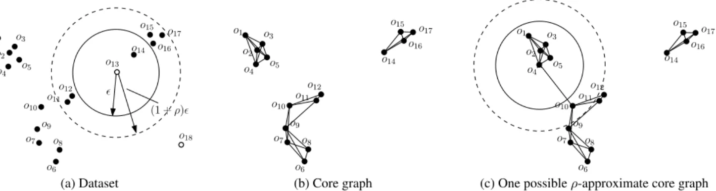
(a) Dataset (b) Core graph (c) One possibleρ-approximate core graph
Figure 2: Illustration of DBSCAN andρ-approximate DBSCAN (ρ= 0.5,MinPts = 3)
MinPts, which can be regarded as a constant. Next, we review how the clusters are formed using graph terminology.
Given a pointp∈P, we useB(p, r)to represent the ball that is centered atp, and has radiusr. The point is said to be acore point
ifB(p, ǫ)covers at leastMinPtspoints ofP(includingpitself); otherwise, it is anon-core point. To illustrate, consider the dataset of 18 points in Figure 2a, whereǫis the radius of the inner solid circle, andMinPts= 3. The core points have been colored black, while the non-core points colored white. The dashed circle can be ignored for the time being.
DBSCAN clusters are defined in two steps. The first one focuses exclusively on the core points, and groups them into preliminary clusters. The second step determines how the non-core points should be assigned to the clusters. Next, we explain the two steps in detail.
Step 1: Clustering Core Points. It will be convenient to imagine an undirectedcore graphGonP—this graph is conceptual and need not be materialized. Specifically, each vertex ofGcorresponds to a distinctcorepoint inP. There is an edge between two core points (a.k.a. vertices)p1, p2if and only ifdist(p1, p2)≤ǫ, where dist(·,·)represents the Euclidean distance between two points. Fig-ure 2b shows the core graph for the dataset of FigFig-ure 2a.
Each connected component (CC) ofGconstitutes a preliminary cluster. In Figure 2b, there are 3 CCs (a.k.a. preliminary clusters). Note that every core point belongs toexactly onepreliminary cluster.
Step 2: Non-Core Assignment. This step augments the preliminary clusters with non-core points. For each non-core pointp, DBSCAN looks at every core pointpcore∈B(p, ǫ), and assignspto the (only)
preliminary cluster containingpcore. Note that, in this manner,p
may be assigned to zero, one, or more than one preliminary cluster. After all the non-core points have been assigned, the preliminary clusters become final clusters.
It should be clear from the above that the DBSCAN clusters are uniquely defined by the parametersǫandMinPts, but they are not necessarily disjoint. A non-core point may belong to multiple clusters, while a core point must exist only in a single cluster. It is possible that a non-core point is not in any cluster; such a point is callednoise.
In Figure 2a, there are two non-core pointso13ando18. Since B(o13, ǫ)coverso14,o13is assigned to the preliminary cluster of o14.B(o18, ǫ), however, covers no core points, indicating thato18is
noise. The final DBSCAN clusters are{o1, o2, ..., o5},{o6, o7, ..., o12},{o13, o14, ..., o17}.
Remark.DBSCAN can also be defined under the notion of “density-reachable”; see [9]. The above graph-based definition is
equiv-alent, perhaps more intuitive, and allows a simple extension to
ρ-approximate DBSCAN, as we will see later.
Hardness of DBSCAN and USEC.It is easy to see that the DB-SCAN clusters on a setPofnpoints can be computed inO(n2)
time, noticing that the core graphGhasO(n2)edges. However,
clever algorithms should produce the clusterswithoutgenerating all the edges, and thus, avoid the quadratic trap. Indeed, whend= 2, the clusters can be computed in onlyO(nlogn)time [11].
It would be highly desired to find an algorithm ofO˜(n)time for
d ≥3, but recently Gan and Tao [10] have essentially dispelled the possibility. They proved anO(n)-time reduction from the unit-spherical emptiness checking (USEC)problemto DBSCAN. In other words, anyT(n)-time DBSCAN algorithm implies that USEC problem can be solved withO(T(n))time.
In USEC, we are given a setSredof red points and a setSblue
of blue points inRd. All the points have distinct coordinates on every dimension. The objective is to determine whether there exist a red pointpredand a blue pointpbluesuch thatdist(pred, pblue)≤1
(the distance threshold 1 can be replaced with any positive value by scaling). The problem has a lower bound ofΩ(n4/3)ford
≥5in a broad class of algorithms [6,7]. Ford= 3and4, beating the bound has been a grand open problem in theoretical computer science, and is widely believed [6] to be impossible. By the reduction of [10], no DBSCAN algorithm can have running timeo(n4/3)ind≥5; ind= 3and 4, this is also true unless unlikely ground-breaking improvements could be made on 3D USEC.
Approximation and the Sandwich Guarantee.Gan and Tao [10] developedρ-approximate DBSCAN, which returns almost the same clusters as exact DBSCAN by offering a strongsandwich guarantee
that will be introduced shortly. In contrast to the high time complex-ity of the latter, the approximate version takes onlyO(n)expected time to compute for any constantρ >0.
Besides the parametersǫandMinPtsinherited from DBSCAN, the approximate version accepts a third parameterρ, which is a small positive constant less than 1, and controls the clustering precision. Its clusters can also be defined in the same two steps as in exact DBSCAN, as explained below.
Step 1: Clustering Core Points.It will also be convenient to follow a graph-based approach. Let us define an undirectedρ-approximate core graphGρon the datasetP—again, this graph is conceptual
and need not be materialized. Each vertex ofGρcorresponds to a
distinct core point inP. Given two core pointsp1, p2, whether or
notGρhas an edge between their vertices is determined as: • The edge definitely exists ifdist(p1, p2)≤ǫ.
• The edge definitely does not exist ifdist(p1, p2)>(1 +ρ)ǫ. • Don’t care, otherwise.
Each preliminary cluster is still a CC, but ofGρ. Unlike the core
graphG,Gρmay not be unique. This flexibility is the key to the
vast improvement in time complexity [10].
To illustrate, consider the dataset of Figure 2a again with theǫ
shown andMinPts = 3, but also withρ= 0.5(the radius of the dashed circle indicates the length of(1 +ρ)ǫ). Figure 2c illustrates a possibleρ-approximate core graph. Attention should be paid to the edge(o4, o10). Note (from the circles in Figure 2c) that ǫ < dist(o4, o10) < (1 +ρ)ǫ—this belongs to the “don’t-care”
case meaning that there may or may not be an edge(o4, o10). If
the edge exists (as in Figure 2c), there are 2 CCs (i.e., preliminary clusters); otherwise, theρ-approximate core graph is the same as in Figure 2b, giving 3 preliminary clusters.
Step 2: Non-Core Assignment. Each non-core pointpmay be as-signed to zero, one, or multiple preliminary clusters. Specifically, letSbe a CC ofGρ. Whetherpshould be added to the preliminary
cluster ofSis determined as:
• Yes, ifShas a core point inB(p, ǫ).
• No, ifShas no core point inB(p,(1 +ρ)ǫ).
• Don’t care, otherwise.
The preliminary clusters after all the assignment constitute the final clusters.
As mentioned,o13ando18are the only two non-core points in
Figure 2a. Whileo18is still a noise point, the case ofo13is more
interesting. First, itmustbe assigned to the preliminary cluster of
o14, just like exact DBSCAN. Second, itmay or may notbe assigned
to the preliminary cluster ofo12(also the cluster ofo14). Either case
is regarded as a correct result.
Sandwich Guarantee. Recall that the clusters of exact DBSCAN are uniquely determined by the parametersǫandMinPts. Now imagine we slightly increaseǫby an amount no more thanρǫ. Have the clusters of DBSCAN changed? If yes, it means that the origi-nal choice ofǫisunstable—clusters are susceptible even to a tiny perturbation toǫ. If no, then the sandwich guarantee asserts that
ρ-approximate DBSCAN returns precisely the same clusters as DB-SCAN. In Figure 2, the clusters changed becauseǫwas deliberately set to be a large value of0.5. In [10], the recommended value for practical data is actually0.001.
We refrain from elaborating on the formal description of the sandwich guarantee at this moment. We will come back to this in Section 6 where we prove that our new “double-approximate” DBSCAN offers just the same guarantee.
Remark.Note, interestingly, that whenρ= 0, there are no “don’t-care” scenarios such thatρ-approximate DBSCAN degenerates into exact DBSCAN. Hence, the former actually subsumes the latter as a special case.
3.
PROBLEM DEFINITION AND STATE OF
THE ART
The Problem of Dynamic Clustering. We now provide a formal formulation of dynamic clustering, using the C-group-by query as the key stepping stone. Our approach is to define the problem in a way that is orthogonal to the semantics of clusters, so that the problem remains valid regardless of whether we have DBSCAN or any of its approximate versions in mind.
LetPbe a set of points inRdthat is subject toupdates, each of which inserts a new point toP, or deletes an existing point fromP. We are given aclustering descriptionwhich specifies correct ways to clusterP. The description is what distinguishes DBSCAN from, e.g.,ρ-approximate DBSCAN.
Suppose that, by the clustering description,C(P)is a legal set of clusters on the current contents ofP. Without loss of generality, assume thatC(P) ={C1, C2, ..., Cx}, wherexis the number of
clusters, andCi(1≤i≤x) is a subset ofP. Note that the clusters
do not need to be disjoint.
Given an arbitrary subsetQofP, acluster-group-by(C-group-by)
querymust return for everyCi∈ C(P)(i∈[1, x]): • Nothing at all, ifCi∩Q=∅
• Ci∩Q, otherwise.
This definition has several useful properties:
• It breaksonlythe points ofQby how they should appear together in the clusters ofP. Points inP\Qare not reported at all, thus avoiding “cheating algorithms” that use “expensive report time” as an excuse for high processing cost.
• WhenQ=P, the query resultQ(P)is simplyC(P).
• All the query results must be based on thesameC(P). This prevents another form of “cheating” when the clustering de-scription permits multiple legal possibilities ofC(P). Specifi-cally, the algorithm can no longer argue that the resultsQ1(P)
andQ2(P)of two queriesQ1andQ2should both be
“cor-rect” becauseQ1(P)is defined on one possibleC(P), while Q2(P)is defined on another. Instead, they must be
consis-tently defined on the sameC(P)—the one output by the query withQ=P.
Our objective is to design an algorithm that is fast in processing both updates and queries. We distinguish two scenarios: (i) semi-dynamic: where all the updates are insertions, and (ii)fully-dynamic, where the updates can be arbitrary insertions and deletions.
We consider that the dimensionalitydis small such that(√d)dis
an acceptable hidden constant. All our theoretical results will carry this constant, and hence, are suitable only for low dimensionality. Our experiments run up tod= 7.
Dynamic Exact DBSCAN [8].Dynamic maintenance of density-based clusters has been studied by Ester et al. [8] for exact DB-SCAN. Next, we review their method—namedincremental DB-SCAN(IncDBSCAN)—assumingMinPts= 1so that all the points ofPare core points. This allows us to concentrate on the main ideas without the relatively minor details of handling non-core points.
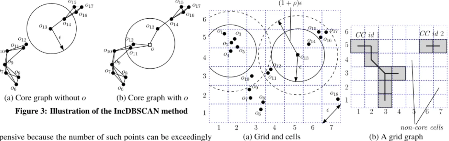
Insertion. Recall that, for exact DBSCAN, the clustersC(P)are uniquely determined by the input parametersǫandMinPts. Given a new pointpnew, the insertion algorithm retrieves all the points in B(pnew, ǫ), and then merges the clusters of those points into one.
The correctness can be seen from the core graphG, where ef-fectively an edge is added betweenpnewand every other point in B(pnew, ǫ)(remember: this view is conceptual, andGdoes not
need to be materialized). Figure 3a shows theGbefore the insertion, which has two CCs. To insert pointoas in Figure 3b, the algorithm finds the pointso11, o12, ando13inB(pnew, ǫ). The two clusters of
those points are merged—the newly added edges(o, o11),(o, o12), (o, o13)in Figure 3b connect the two CCs into one.
In merging the clusters, IncDBSCAN does not modify the cluster ids of the points in the affected clusters, which can be prohibitively
o6 o7 o8 o9 o10 o11 o12 o14 o15 o16 o17 o13 ǫ o6 o7 o8 o9 o10 o11 o12 o14 o15 o16 o17 o13 o
(a) Core graph withouto (b) Core graph witho
Figure 3: Illustration of the IncDBSCAN method
expensive because the number of such points can be exceedingly high. Instead, it remembers the “merging history” of the cluster ids.
Deletion.The deletion algorithm, in general, reverses the steps of insertion, except for a breadth first search (BFS) that is needed to judge whether (and how) a cluster has split into several.
Letpoldbe the point being deleted. IncDBSCAN retrieves all the
points inB(pold, ǫ). In (the conceptual)G, all the edges between
such points andpoldare removed, after which the CC ofpoldmay
or may not be broken into separate CCs (e.g., in Figure 3b, the CC is torn into two only ifo13,o14, orois deleted). To find out,
the deletion algorithm performs as many threads of BFS onG
as the number of points inB(pold, ǫ). If two threads “meet up”,
they are combined into one because they must still be in the same CC. As soon as only one thread is left, the algorithm terminates, being sure that no cluster split has taken place. Otherwise, the remaining threads continue until the end, in which case each thread has enumerated all the points in a new cluster that is spawned by the deletion. All those points can now be labeled with the same cluster id.
For example, suppose that we deleteoin Figure 3b, which starts three threads of BFS fromo11, o12ando13, respectively. The
re-sulting core graph reverts back to Figure 3a. The threads ofo11
ando12meet up into one, which eventually traverses the entire CC
containingo11ando12. Similarly, the other thread traverses the
entire CC containingo13.
When a thread of BFS needs the adjacent neighbors of a pointp1
inG, the algorithm finds all the other pointsp2∈B(p1, ǫ)through
arange query[3,12]. Every suchp2is an adjacent neighbor ofp1.
This essentially “fetches” the edge betweenp1andp2.
Query.The algorithm of [8] can easily answer a C-group-by query
Qby grouping the points ofQby their cluster ids (some ids need to be obtained from the merging history).
Drawbacks of IncDBSCAN.Both insertion and deletion start with a range query to extract the points inB(p, ǫ), which are called the
seed points[8]. The query is expensive whenpfalls in a dense region ofP where there are many seed points. The issue is more serious in a deletion, because multiple range queries are needed to perform BFS. The worst situation happens in a cluster split, where the number of range queries is simply huge.
4.
THE OVERALL FRAMEWORK
All the DBSCAN variants (including the new one to be proposed in Section 6.2) accept parametersǫ,MinPts, andρ(for exact DB-SCAN,ρ = 0). This permits us to extract a common structural framework behind all our solutions, as we describe in this section.
o6 o7 o8 o9 o10 o11 o12 o13 o14 o15 o16 o17 o1 o2 o3 o4 o5 ǫ (1 +ρ)ǫ ǫ 1 2 3 4 5 6 7 1 2 3 4 5 6 o18 1 2 3 4 5 6 7 1 2 3 4 5 6 CC id1 CC id2 non-core cells
(a) Grid and cells (b) A grid graph
Figure 4: Our grid-graph framework (MinPts = 3)
The components of the framework will be instantiated differently in later sections for individual variants.
4.1
A Grid Graph Approach
The key idea behind our framework is to turn dynamic clustering into the problem of maintaining CCs (connected components) of a special graph.
Grid and Cells.We impose an arbitrary gridDin the data spaceRd,
where each cell is ad-dimensional square with side lengthǫ/√don every dimension. This ensures that any two points in the same cell are within distance at mostǫfrom each other.
Given a cellcofD, we denote byP(c)the set of points inPthat
are covered byc. We callc
• Anon-empty cellifP(c)contains at least one point.
• Acore cellifP(c)contains at least one core point.
• Adense cellif|P(c)| ≥MinPts, and asparse cellif1≤ |P(c)|<MinPts.
Given two cellsc1, c2, we say that they areǫ-closeif the smallest
distance between the boundary ofc1and that ofc2is at mostǫ.
Consider for instance the grid in Figure 4a, imposed on a setPof 18 points. Again, the radii of the solid and dashed circles indicate
ǫand(1 +ρ)ǫ, respectively; andMinPts= 3. The only non-core points areo13ando18. The core cells are shaded in Figure 4b. The
non-core cells are(5,4)and(7,2); note that the minimum distance between the two cells isǫ—hence, they areǫ-close.
Grid Graph. In agrid graphG = (V,E),Vis the set of core
cells ofD, whileEis a set of edges satisfying the followingCC requirement:
Letp1, p2be two core points ofP, andc1(orc2, resp.) be
the core cell that containsp1(orp2, resp.). Then,p1andp2
are in the same clusterif and only ifc1andc2are in the same
CC ofG.
The above requirement is fulfilled by using the following rules to decide ifEshould have an edge between two core cellsc1, c2∈V: • Yes, if there is a pair of core points(p1, p2)∈P(c1)×P(c2)
satisfyingdist(p1, p2)≤ǫ.
• No, if there isnopair of core points(p1, p2)∈P(c1)×P(c2)
satisfyingdist(p1, p2)≤(1 +ρ)ǫ. • Don’t care, otherwise.
⇒ + + − + + − + + − updates onP core-status structure core cell updates
GUM
edge changes
CC structure
Figure 5: Flow of updates in our structures
Gdiffers significantly from the core graphGand theρ-approximate core graph ofGρas reviewed in Section 2.Ghas at mostnvertices
because there are at mostnnon-empty cells. IfG has an edge
between core cellsc1, c2, they must beǫ-close. A core cell can
haveO ǫ ǫ/√d
d
=O((√d)d) =O(1)ǫ-close core cells
(re-call that our target is low dimensionality). Hence,Gcan have only
O(n)edges, which makes it suitable for materialization when the dimensionalitydis low.
Figure 4b demonstrates the grid graph for the dataset in Figure 4a. Note that the edge between cells(2,4)and(3,3)fall into the don’t-care case, becauseǫ <dist(o4, o10)≤(1 +ρ)ǫ. ThatGsatisfies
the CC requirement can be seen together with theρ-approximate core graph in Figure 2c. For example,o3ando6are in the same
cluster, consistent with the fact that cells(2,5)and(3,1)are in the same CC ofG. Conversely, as cells(2,5)and(6,5)are in different CCs ofG, we knowo3ando14must be in different clusters.
4.2
Query Algorithm
All our solutions actually use the same algorithm to answer C-group-by queries. We explain the algorithm in this subsection, as well as the necessary data structures.
Core-Status Structure.We explicitly record whether each point inP is a core or non-core point. This structure maintains these core-status labels under insertions and deletions of the points inP. A semi-dynamic structure only needs to support insertions.
ρ-Approximateǫ-Emptiness.Given a pointqand a core cellc, an
emptiness queryempty(q, c)returns:
• 1, ifP(c)has a core pointpsatisfyingdist(p, q)≤ǫ.
• 0, ifnocore pointp∈P(c)satisfiesdist(p, q)≤(1 +ρ)ǫ.
• 1 or 0 (don’t care), otherwise.
As a furthermore requirement, if the output is 1, the query must also return aproof pointp∈P(c), which is a core point satisfying
dist(q, p)≤(1 +ρ)ǫ.
For example, forq=o13andc=cell(6,5), the emptiness query
must return 1 due to the presence ofo14. Ifcchanges to cell(3,2),
then the query must return 0. Settingq =o4andc =cell(3,3)
gives a don’t-care case.
We maintain anemptiness structureon every core cellcto support (i) such queries efficiently, and (ii) insertions/deletions of core points inP(c). Deletions are not needed if the structure is semi-dynamic.
CC Structure.We maintain a structure onGto support:
• EdgeInsert(c1, c2): Add an edge between core cellsc1, c2to G.
• EdgeRemove(c1, c2): Remove the aforementioned edge. • CC-Id(c): Given a core cellc, return a unique id of the CC of
Gwherecbelongs.
If a CC structure is semi-dynamic, it does not need to support
EdgeRemove.
C-Group-By Query.Next, we clarify how to answer a C-group-by queryQ. DivideQinto a setQ1of core points, and a setQ2of
non-core points. This takesO(|Q|)time using the core-status structure. For every core pointq∈Q1, we retrieve the core cellccoveringq,
performCC-Id(c), and set the CC id as the cluster id ofq. A non-core pointq∈Q2, on the other hand, is “snapped” to the
nearby core cells. Again, obtain the cellccoveringq. Ifcis a core cell, assign the cluster idCC-Id(c)toq. In any case, we enumerate all theǫ-close core cellsc′ofc. For everyc′, issue an emptiness
queryempty(q, c′). If the emptiness query returns 1, assign the
output ofCC-Id(c′)as a cluster id ofq. Note thatqmay get assigned
multiple cluster ids.
We can now group the points inQby cluster id. A non-core point belongs to as many groups as the number of its distinct cluster ids; if a non-core point has no cluster ids, it is a noise point.
ConsiderQ = {o13, o14, o8}in the dataset of Figure 4a. Q1
includes core pointso14ando8, which are in cells(6,5)and(3,2),
respectively. InvokingCC-Idon(6,5)returns 2 (see Figure 4b), while doing so to(3,2)returns 1. Q2has only a single non-core
point, in cell(5,4), whoseǫ-close core cells are(4,3),(3,3),(3,2),
(6,5), and(7,5). We perform an emptiness query usingo13on each
of those 5 cells. Suppose that the emptiness queries on(4,3)and
(6,5)return 1, while the others 0. We thus assign two distinct CC ids too13: 1 and 2. The final result of the C-group-by query is
therefore{o14, o13}, and{o8, o13}.
4.3
Graph Maintenance
To guarantee correctness, we must keep the grid graphG
up-to-date along with the insertions and deletions on the underlying datasetP. This is accomplished through the collaboration of the core-status structure, GUM (see below), and the CC structure.
Graph Update Module (GUM).This module is responsible for maintaining the vertices and edges inG.
Remark. Figure 5 illustrates the data flow in the internal work-ings of our update mechanism. The point insertions and deletions inP are fed into the core-status structure, which informs GUM about which cells have turned into core/non-core cells. Utilizing such information, GUM updates Gby generating the necessary
edge changes, which are passed to the CC structure for properly maintaining the CCs ofG.
Overall, our design will focus on GUM and the core-status struc-ture. CC and emptiness structures have been well-studied in graph theory and computational geometry, respectively; it suffices to plug in the best existing structures suiting our purposes.
5.
SEMI-DYNAMIC ALGORITHMS
This section presents maintenance algorithms for exact/approximate DBSCAN clustering when all the updates are insertions. We will do so by specializing the framework of the last section.
The Core-Status Structure. For each non-core point p ∈ P, we remember avicinity countvincnt(p)which equals the num-ber of points ofP covered byB(p, ǫ). By non-core definition,
vincnt(p) < MinPts. Oncevincnt(p)reachesMinPts, p be-comes a core point, after which we no longer keep track of such a count.
Let us see how to maintain the above information when a new pointpnewis inserted. Letcnewbe the cell ofDthat containspnew.
We start by checking ifpnewis a core point as follows:
1 Ifcnewis dense,pnewmust a core point (all the points incnew
are within distanceǫfrompnew).
2 Otherwise, we simply enumerate all theO(1)ǫ-close cells
cofcnew, and calculate the distances frompnew to all the
points inP(c). This way, we obtain the precise number of points inB(pnew, ǫ), noticing that any point within distanceǫ
frompnewmust be in anǫ-close cell. The core-status ofpnew
can now be decided.
The appearance ofpnewmay increase the vicinity countvincnt(p)
of some non-core pointsp. Suchpmust be covered in cellscthat are (i) sparse, and (ii)ǫ-close tocnew. We find all these points by
simply visiting theP(c)of all suchc.
GUM.In general, whenever we have a new core pointpcore(it may
bepnew, or a pointpthat just has itsvincnt(p)increased),Gmay
need to be updated. Letccorebe the cell coveringpcore. Ifccorejust
became a core cell, we add it intoV. In any case, new edges are
potentially added toEas follows:
1 For everyǫ-close cellcofccorethat currently has no edge
withccoreinG
1.1 Perform an emptiness queryempty(pcore, c).
1.2 If the query returns 1, add(c, ccore)toEand call
EdgeIn-sert(c, ccore).
Performance Guarantees.Using the best CC and emptiness struc-tures under the semi-dynamic scheme, we prove in the appendix:
THEOREM 1. For any fixed dimensionalitydand fixed constant
ρ >0, there is a semi-dynamicρ-approximate DBSCAN algorithm that processes each insertion inO˜(1)amortized time, and answers a C-group-by queryQinO˜(|Q|)time.
The same insertion and query efficiency can also be achieved in 2D space for exact DBSCAN.
6.
DYNAMIC HARDNESS AND DOUBLE
APPROXIMATION
We now come to perhaps the most surprising section of the pa-per. Recall thatρ-approximate DBSCAN was proposed to address the computational hardness of DBSCAN onstaticdatasets. In Section 6.1, we will show that theρ-approximate version suffers from the same hardness onfully dynamicdatasets. Interestingly, the culprit this time is the definition of core point. This motivates the proposition ofρ-double-approximateDBSCAN in Section 6.2, where we also prove that the new proposition has a sandwich guar-anteeas strong astheρ-approximate version.
6.1
Hardness of Dynamic
ρ
-Approximation
USEC with Line Separation.Next, we introduce theUSEC with line separation(USEC-LS)problem, which has a subtle connection withρ-approximate DBSCAN, as shown later.
pred pblue
1
pred pblue p′(dummy)
(a) USEC-LS (b) Reduction to dynamic clustering
Figure 6: Illustration of our hardness proof
In USEC-LS, we are given a setSredof red points and a setSblue
of blue points inRd, which are separated by ad-dimensional plane ℓperpendicular to the first dimension, such that all the red points are on one side ofℓ, and all the blue points on the other. All the points have distinct coordinates on the first dimension. The objective, as with USEC (see Section 2), is to determine whether there exist
pred ∈Sredandpblue ∈Sbluesuch thatdist(pred, pblue)≤1. We
definen=|Sred|+|Sblue|. Figure 6a shows an example where the
answer is “yes”.
Recall from Section 2 that USEC is computationally hard. In the appendix, we prove that this is also true for USEC-LS:
LEMMA 1. If we can solve USEC-LS ino(n4/3)time, then we
can solve USEC ino(n4/3)time.
Dynamic Hardness. Suppose that we have aρ-approximate DB-SCAN algorithm that handles an update (insertion/deletion) in
Tupd(n)amortized time, and answers a C-group-by query with |Q|= 2inTqry(n)amortized time. Then:
LEMMA 2. We can solve the USEC-LS problem inO(n·(Tupd(n)+ Tqry(n))time.
PROOF. Letxbe the coordinate where the separation planeℓ
in USEC-LS intersects dimension 1. Without loss of generality, let us assume that the red points are on theleftofℓ, i.e., having coordinates less thanxon dimension 1. Conversely, the blue points are on therightofℓ. We solve USEC-LS using the given dynamic
ρ-approximate DBSCAN algorithmAas follows.
1. Initialize aρ-approximate DBSCAN instance withǫ= 1,
MinPts= 3, and an arbitraryρ≥0. LetPbe the input set, which is empty at this moment.
2. UseAto insert all the red points intoP.
3. For every blue pointp= (x1, x2, ..., xd)(hence,x1 > x),
carry out the following steps: 3.1 UseAto insertpintoP.
3.2 UseAto insert a dummy pointp′= (x
1+ 1, x2, ..., xd)
intoP. That is,p′has the same coordinates aspon all
dimensionsi ∈ [2, d], except for the first dimension wherep′has coordinatex
1+ 1. See Figure 6b for an
illustration (wherep=pblue).
3.3 UseAto answer a C-group-by query withQ={p, p′}.
If the query returns the same cluster id forpandp′,
terminate the algorithm, and return “yes” to the USEC-LS problem.
3.4 UseAto deletep′andpfromP.
The running time of the algorithm isO(n·(Tupd(n) +Tqry(n))
because we issue at most2ninsertions and2ndeletions, as well as
nqueries, in total. Next, we prove that the algorithm is correct. Consider Lines 3.1-3.4. A crucial observation is that the dummy pointp′must be a non-core point, becauseB(p′, ǫ)contains only
two pointsp, p′. Therefore,p′andpare placed into the same cluster
byρ-approximate DBSCANif and only ifpis a core point. However,
pis a core point if and only ifB(p, ǫ)covers at least 3 points, which must includep,p′, and at least one pointp′′on the other side of ℓ—red pointp′′and blue pointpare therefore within distance 1.
It is now straightforward to verify that our algorithm always returns the correct answer for USEC-LS.
THEOREM 2. For anyρ≥0and any dimensionalityd≥3, any
ρ-approximate DBSCAN algorithm must incurΩ(n1/3)amortized
time either to process an update, or to answer a C-group-by query (even if|Q|= 2), unless the USEC problem inRdcould be solved ino(n4/3)time.
PROOF. Suppose that the algorithm were able to process an up-date and a query both ino(n1/3)amortized time. By Lemma 2, we
would solve USEC-LS ino(n4/3)time which, by Lemma 1, means that we would solve USEC ino(n4/3)time.
As explained in Section 2, for USEC, a lower bound ofΩ(n4/3)is
known [7] ind≥5, whereas beating theO(n4/3)bound ind= 3,4
is a major open problem in theoretical computational geometry, and believed to be impossible [6].
This is disappointing because DBSCAN succumbing to the hard-ness of USEC was what motivatedρ-approximate DBSCAN. Theo-rem 2 shows that the latter suffers from the same hardness when both insertions and deletions are allowed! Note that the theorem does not apply to the semi-dynamic update scheme because the deletions at Line 3.4 are essential. In fact, Theorem 1 already proved that effi-cient semi-dynamic algorithms exist forρ-approximate DBSCAN.
Finally, it is worth pointing out that Theorem 2 holds even for
ρ= 0, i.e., it is applicable to exact DBSCAN as well.
6.2
ρ
-Double-Approximate DBSCAN and
Sandwich Guarantee
The New Proposition. To enable both (fully-dynamic) update and query efficiency, we proposeρ-double-approximate DBSCAN, which takes the same parametersǫ,MinPts, andρasρ-approximate DBSCAN. Whether a pointp∈Pis a core point is now decided in a relaxed manner:
• Definitely a core point if B(p, ǫ) covers at leastMinPts
points ofP.
• Definitely not a core point ifB(p,(1 +ρ)ǫ)covers less than
MinPtspoints ofP.
• Don’t care, otherwise.
A good example to illustrate this is pointo13in Figure 4a. Since B(o13, ǫ)covers2<MinPts = 3points,o13is not a core point
under exact orρ-approximate DBSCAN. Under double approxima-tion, however, it falls into the don’t-care case forρ= 0.5, because
B(p,(1 +ρ)ǫ)covers 7 points.
The clusters ofρ-double-approximate DBSCAN are defined by the same two-step approach ofρ-approximate DBSCAN (see Sec-tion 2), but with respect to the above core-point semantics. Swaying
o13into a core point, Figure 7a shows theρ-double-approximate
core graph (defined precisely as theρ-approximate version), while Figure 7b gives the corresponding grid graph.
o6 o7 o8 o9 o10 o11 o12 o14 o15 o16 o17 o1 o2 o3 o4 o5 o13 1 2 3 4 5 6 7 1 2 3 4 5 6 CC id1 CC id2
(a) One possibleρ-double-approx (b) Grid graph core graph
Figure 7: Illustration ofρ-double approximation Sandwich Guarantee.Recall that this is an attractive feature ofρ -approximate DBSCAN. Next, we prove thatρ-double-approximate DBSCAN provides just the same guarantee. Following the style of [10], we define:
• C1as the set of clusters of exact DBSCAN with parameters (ǫ,MinPts).
• C2as the set of clusters of exact DBSCAN with parameters (ǫ(1 +ρ),MinPts).
• Cas a set of clusters that is a legal result ofρ-double-approximate
DBSCAN with parametersǫ,MinPts, andρ. Then, the sandwich guarantee is:
THEOREM 3. The following statements are true: (i) For any clusterC1∈C1, there is a clusterC∈C such thatC1⊆C, and
(ii) for any clusterC ∈ C, there is a clusterC2 ∈C2such that C⊆C2.
The proof can be found in the appendix. Note that the theorem is purposely worded exactly the same as Theorem 3 of [10].
7.
FULLY DYNAMIC ALGORITHMS
This section presents our algorithms for maintainingρ -double-approximate DBSCAN clusters under both insertions and deletions (again, exact DBSCAN is captured withρ= 0). We will achieve the purpose by instantiating the general framework in Section 4. The reader is reminded that the core-point definition has changed to the one in Section 6.2.
7.1
Approximate Bichromatic Close Pair
We now take a short break from clustering to discuss a computa-tional geometry problem which we name theapproximate bichro-matic close pair(aBCP)problem. In this problem, we have two disjoint axis-parallel squaresc1, c2inRd. There is a setS(c1)of
points inc1, and a setS(c2)of points inc2. The two sets are subject
to insertions and deletions. Letǫandρbe positive real values. We are asked to maintain awitness pairof(p∗
1, p∗2)such that • It may be an empty pair (i.e.,p∗
1andp∗2are null). • If it is not empty, we must havedist(p∗
1, p∗2)≤(1 +ρ)ǫ. • The pair must not be empty, if there exist a pointp1∈S(c1)
and a pointp2∈S(c2)such thatdist(p1, p2)≤ǫ. Note that
the pair doesnothave to be(p1, p2)though.
We have at our disposal an emptiness structure (as defined in Section 4.2) on each cell, so that an emptiness query(q, c)with
c=c1orc2can be answered with costO˜(τ)for some time function τ. The objective is to minimize the cost of (i) finding an initial witness pair, and (ii) maintaining the pair along with updates in
LEMMA 3. For the aBCP problem, an initial witness pair can be found inO˜(τ·min{|S(c1)|,|S(c2)|})time. After that, the pair
can be maintained byO˜(τ)amortized time when a point is inserted or deleted inS(c1)orS(c2).
The proof can be found in the appendix.
7.2
Edges in the Grid Graph and aBCP
Returning toρ-double-approximate DBSCAN clustering, let us recall that in the grid graphG, if there is an edge between core
cellsc1andc2, then the two cells must beǫ-close. Such an edge
may disappear/re-appear as the core points ofP(c1) andP(c2)
are deleted/inserted. Maintaining this edge can be regarded as an instance of the aBCP problem, whereS(c1)is the set of core points
inP(c1), andS(c2)is the set of core points inP(c2)—the edge
exists if and only if the witness pair is not empty!
We run a thread of the aBCP algorithm of Lemma 3 on every pair ofǫ-close core cellsc1andc2. Those threads will be referred to as
theaBCP instancesofc1(orc2). Whenever the edge betweenc1
andc2(re-)appears, we callEdgeInsert(c1, c2)of the CC structure;
whenever it disappears, we callEdgeRemove(c1, c2).
7.3
The Core-Status Structure
Given a pointq, anapproximate range count query[10] returns an integerkthat falls between|B(q, ǫ)|and|B(q,(1 +ρ)ǫ)|. The query can be answered inO˜(1)time by a structure that can be updated inO˜(1)time per insertion and deletion [16]. Under the relaxed core-point definition ofρ-double-approximation, whether a pointp∈Pis a core point can be decided directly by issuing such a query withp. If the query returnsk, we declarepa core point if and only ifk≥MinPts.
Leveraging this fact, next we describe how to explicitly update the core-status of all points inPalong with insertions and deletions:
• To insert a pointpnew in cellcnew, we first check whether pnewitself is a core point. Remember that the insertion may
turn some existing non-core points into core points. To iden-tify such points, we look at each of theO(1)ǫ-close sparse cellscofcnew. Simply check all the pointsp∈P(c)to see
ifpis currently a core point.
• The deletion of a pointpold from cellcold may turn some
existing core points into non-core points. Following the same idea in insertion, we look at everyǫ-close sparse cellcofcold,
and check all the pointsp∈P(c)for their current core status.
7.4
GUM
When a pointpcore(say, in cellccore) has turned into a core point,
we check whetherccoreis already inV:
• If so, simply insertpcoreinto every aBCP instance (Lemma 3)
ofccore—as explained in Section 7.2, this properly maintains
the edges ofccore.
• Otherwise, it must hold that|P(ccore)| ≤MinPts=O(1).
We addccore toV. Then, for everyǫ-close core cellcof ccore, decide whether to create an edge betweencandccore
by using the algorithm of Lemma 3 to find an initial witness pair (thereby starting the aBCP instance onccoreandc).
Consider now the scenario where a core pointpin cellccorehas
turned into a non-core point. Ifccoreis still a core cell, we removep
from all the aBCP instances ofccore. Otherwise, we simply remove ccorefromV, and destroy all its aBCP instances.
7.5
Performance Guarantees
Utilizing the best CC and emptiness structures under the fully-dynamic scheme, we prove in the appendix our last main result:
THEOREM 4. For any fixed dimensionalitydand fixed constant
ρ > 0, there is a fully-dynamicρ-double-approximate DBSCAN algorithm that processes each insertion and deletion inO˜(1) amor-tized time, and answers a C-group-by queryQinO˜(|Q|)time.
The same update and query efficiency can also be achieved in 2D space for exact DBSCAN.
8.
EXPERIMENTS
Section 8.1 describes the setup of our empirical evaluation. Then, Sections 8.2 and 8.3 report the results on semi-dynamic and fully-dynamic algorithms, respectively.
8.1
Setup
Workload. We evaluate a clustering algorithm by its efficiency in processing aworkload, which is a mixed sequence of updates and queries. Each update or query is collectively referred to as an
operation. A workload is characterized by several parameters:
• N: the total number of updates.
• %ins: the percentage of insertions. In other words, the
work-load hasN·%insinsertions, andN(1−%ins)deletions. This
parameter is fixed to1in semi-dynamic scenarios.
• fqry: the query frequency, which is an integer controlling how often a C-group-by query is issued.
The production of a workload involves 3 steps, as explained below.
Step 1: Insertions. The sequence of insertions is obtained by first generating a “static dataset” ofI = N ·%ins points, and then,
randomly permuting these points (i.e., if a point stands at thei-th position, it is thei-th inserted). We generate static datasets whose clusters are the outcome of a “random walk with restart”, as was the approach suggested in [10], and will be reviewed shortly. Note that the random permutation mentioned earlier allows the clusters to form up even at an early stage of the workload.
Thedata spaceis ad-dimensional square that has range[0,105]
on each dimension. A static dataset is created using theseed spreader technique in [10], which generates around10clusters and0.0001·Inoise points as follows. First, place a spreader at a random locationpof the data space. At eachtime tick, the spreader adds to the dataset a point that is uniformly distributed inB(p,25). Whenever the spreader has generated100points while stationed at the samep, it is forced to move towards a random direction by a distance of 50. Finally, with probability10/(0.9999I), the spreader “restarts” by jumping to another random location of the data space. Regardless of whether a restart happens, the current time tick fin-ishes, and the next one starts. The spreader works for0.9999Itime ticks (thus producing0.9999Ipoints). After that,0.0001·Irandom points are added to the dataset as noise.
Step 2: Deletions. First, append to the insertion sequenceD = N−Ideletiontokens, where each token is simply a “place-holder”
parameter value
d 2,3,5,7
ǫ 50d,100d,200d,400d,800d %ins 23,45,5/6,89,1011
fqry 0.01N,0.02N,0.03N, ...,0.1N
Semi-Approx 2d-Semi-Exact IncDBSCAN 1 10 102 103 0 2 5 8 11
number of operations (million) average cost per operation (microsec)
(a) Average operation cost vs. time
10 102 103 104 105 0 2 5 8 11
number of operations (million) maximum update cost (microsec)
(b) Max update cost vs. time
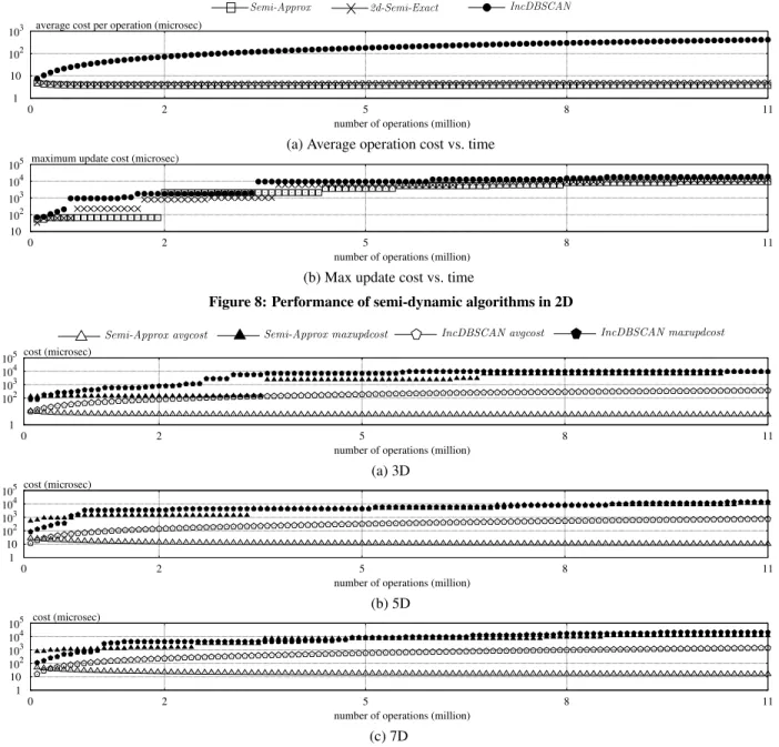
Figure 8: Performance of semi-dynamic algorithms in 2D
Semi-Approx avgcost Semi-Approx maxupdcost IncDBSCAN avgcost IncDBSCAN maxupdcost
1 102 103 104 105 0 2 5 8 11
number of operations (million) cost (microsec) (a) 3D 1 10 102 103 104 105 0 2 5 8 11
number of operations (million) cost (microsec) (b) 5D 1 10 102 103 104 105 0 2 5 8 11
number of operations (million) cost (microsec)
(c) 7D
Figure 9: Performance of semi-dynamic algorithms ind≥3dimensions
into which we will later fill a concrete point to delete. Then, ran-domly permute the resulting sequence (which has lengthN). Check whether the permutation isbad, namely, if any of its prefixes has more tokens than insertions. If so, we attempt another random permutation until agoodone is obtained.
Now we have a good sequence of insertions and deletion tokens. To fill in the tokens, scan down the sequence, and add each inserted point intoS, until coming across the first token. Select a random point inSas the one deleted by the token, and then remove the point fromS. The scan continues in this fashion until all the tokens have been filled.
Step 3: Queries.We simply insert a C-group-by query after every
fqry updates in the sequence. Recall that the query specifies a parameterQ, which is generated as follows. LetSbe the set of “alive” points that have been inserted, but not yet deleted before the query. We first decide the value of|Q|by choosing an integer
uniformly at random from[2,100]. Then,Qis populated by random sampling|Q|points fromSwithout replacement.
DBSCAN Algorithms.Our experimentation examined:
• IncDBSCAN [8]: the state-of-the-art dynamic algorithm for exact DBSCAN, as reviewed in Section 3.
• 2d-Semi-Exact: our semi-dynamic algorithm in Theorem 1 for exact DBSCAN in 2D space.
• Semi-Approx: our semi-dynamic algorithm in Theorem 1 for
ρ-approximate DBSCAN ind-dimensional space withd≥2.
• 2d-Full-Exact: our fully-dynamic algorithm in Theorem 4 for exact DBSCAN in 2D space.
• Double-Approx: our fully-dynamic algorithm in Theorem 4 forρ-double-approximate DBSCAN ind-dimensional space withd≥2.
All the algorithms were implemented in C++, and compiled with gcc version 4.8.4.
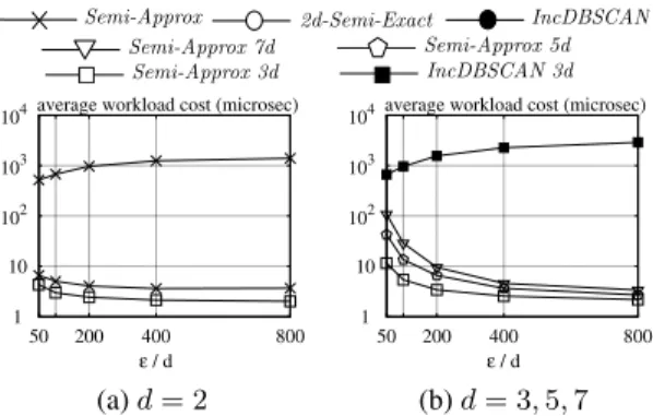
Semi-Approx 2d-Semi-Exact IncDBSCAN Semi-Approx 7d IncDBSCAN 7d Semi-Approx 5d IncDBSCAN 5d Semi-Approx 3d IncDBSCAN 3d 1 10 102 103 104 50 200 400 800 ε / d
average workload cost (microsec)
1 10 102 103 104 50 200 400 800 ε / d
average workload cost (microsec)
(a)d= 2 (b)d= 3,5,7
Figure 10: Semi-dynamic performance vs.ǫ
Parameters and Machine.We fixedNto 10 million, namely, each workload contains this number of updates. The value ofMinPts
in all the DBSCAN variants was 10. The value ofρin the approxi-mate variants was set to0.001, under whichρ-double-approximate DBSCAN is required to return precisely the same clusters asρ -approximate DBSCAN.
The other parameters were varied in different experiments. Their values are as shown in Table 2; unless otherwise stated, a parameter was set to its default as shown in bolds. Note that%ins = 5/6
indicates on average 1 deletion every 5 insertions.
Finally, all the experiments were run on a machine equipped with an Intel Core i7-6700 CPU @ 3.40GHz×8 and 16GB memory. The operating system was Linux (Ubuntu 14.04.1).
8.2
Semi-Dynamic Results
This subsection will focus on insertion-only workloads. Con-sider executing an algorithm on such a workload. We define the algorithm’saverage costas a function of time: avgcost(t) = 1
t Pt
i=1cost[i], wherecost[i]is the overhead of the algorithm in
processing thei-th operation of the workload. Similarly, define the algorithm’smax update costas:maxupdcost(t) = maxxi=1updcost[i],
where (i)xis the number of updates by the end of thet-th oper-ation, and (ii)updcost[i]is the overhead of the algorithm for the
i-th update. Notice that query time is registered inavgcostbut not
maxupdcost.
Focusing on 2D space, Figure 8a plots the average cost of IncDB-SCAN,2d-Semi-Exact, andSemi-Approx, whereas Figure 8b plots their max update cost. 2d-Semi-ExactandSemi-Approxfinished the workload significantly faster thanIncDBSCAN, achieving an improvement of two orders of magnitude! Moreover, while the aver-age cost ofIncDBSCANdeteriorated continuously, the performance of2d-Semi-ExactandSemi-Approxremained stable throughout the workload. This is expected becauseIncDBSCANmust perform a range query per insertion (see Section 3), which tends to retrieve more data points as time progresses. Our solutions do not suffer from this drawback.
Turning to 3D space—where the competing methods are IncDB-SCANandSemi-Approx— Figure 9a compares their average cost and max update cost simultaneously. Figures 9b and 9c present the same results ford= 5and7, respectively. In all dimensionali-ties,Semi-Approxconsistently outperformedIncDBSCANby a wide margin even in logarithmic scale.
Interestingly, all the methods exhibited similar behavior when it comes to themaxupdcost metric. We will return to this issue later when we discuss the fully dynamic scenario, where contrasting phenomena will be observed.
Semi-Approx 2d-Semi-Exact IncDBSCAN Semi-Approx 7d IncDBSCAN 7d Semi-Approx 5d IncDBSCAN 5d Semi-Approx 3d IncDBSCAN 3d 1 10 102 103 104 0.1 0.4 0.6 0.8 1
query frequency (million) average workload cost (microsec)
1 10 102 103 104 0.1 0.4 0.6 0.8 1 query frequency (million) average workload cost (microsec)
(a)d= 2 (b)d= 3,5,7
Figure 11: Semi-dynamic performance vs.fqry
We define an algorithm’saverage workload costasavgcost(W), whereW is the total number of operations in the workload of con-cern. The next experiment demonstrates the effect ofǫon the cost of cluster maintenance—as discussed in [1,10], an algorithm of density-based clustering should be able to find clusters at differ-entgranularitiesofǫ. Figure 10 shows the average workload cost of each applicable method as a function ofǫ, ford = 2,3,5,7, respectively. It is evident that IncDBSCAN became prohibitively expensive asǫincreases. On the other hand, our solutions actually performed even better for largerǫ! This is not surprising because a greaterǫactuallyreducesthe number of edges in the grid graph, which in turn leads to substantial cost savings.
We conclude this subsection by giving the average workload cost of all methods as a function offqryin Figure 11. In general, query
cost is negligible compared to update overhead.
8.3
Fully-Dynamic Results
We now proceed to evaluate the algorithms that can handle both insertions and deletions. Our strategy is similar to that in the previ-ous subsection.Average costandmax update costare defined in the same way as before, except that operations/updates obviously also include deletions here.
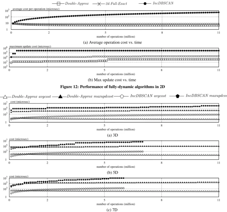
Figure 12 shows the results in experiments corresponding to those in Figure 8, with respect toIncDBSCAN,2d-Full-Exact, and Double-Approx. Similarly, Figure 13 corresponds to Figure 9, with respect toIncDBSCANandDouble-Approx. As before, our solutions were two orders of magnitude faster thanIncDBSCANin average cost. What is new, however, is that they also improvedIncDBSCANby nearly 10 times in max update cost as well!
What has triggered the separation inmaxupdcost? The hardness of deletions! Recall from Section 3 thatIncDBSCANrequires only one range query (to find the seed objects) in an insertion, whereas in a deletion, it demands multiple—actually perhaps many—such queries to perform BFS. This stands in sharp contrast to Double-Approx, which completely gets rid of BFS by novel ideas, in par-ticular, deploying an aBCP algorithm (Lemma 3) to convert cluster maintenance to updating the CCs of the grid graph (which has only
O(n)edges). Inall scenarios, our algorithms ensured processing an update in less than0.1seconds! The reader may have noticed thatIncDBSCANdid not finish the 5D and 7D workloads. Indeed, we terminated it after 3 hours when its deficiencies had become apparent.
Figure 14 presents the results that are the counterparts of Fig-ure 10, confirming thatIncDBSCANis essentially inapplicable for largeǫ. Note, again, that this method has no results ford= 5and7.
Double-Approx 2d-Full-Exact IncDBSCAN 1 10 102 103 0 2 5 8 11
number of operations (million) average cost per operation (microsec)
(a) Average operation cost vs. time
102 103 104 105 106 0 2 5 8 11
number of operations (million) maximum update cost (microsec)
(b) Max update cost vs. time
Figure 12: Performance of fully-dynamic algorithms in 2D
Double-Approx avgcost Double-Approx maxupdcost IncDBSCAN avgcost IncDBSCAN maxupdcost
1 103 105 107
0 2 5 8 11
number of operations (million) cost (microsec) (a) 3D 1 103 105 107 0 2 5 8 11
number of operations (million) cost (microsec) (b) 5D 1 103 105 107 0 2 5 8 11
number of operations (million) cost (microsec)
(c) 7D
Figure 13: Performance of fully-dynamic algorithms ind≥3dimensions
The last set of experiments inspected the average workload cost of these algorithms as the insertion percentage increased from2/3
to10/11. The results are reported in Figure 15. In general, the efficiency of each method improved as insertions accounted for a higher percent of the workload. Our new algorithms were the clear winners in all situations.
9.
CONCLUSIONS
This paper has presented a systematic study on dynamic den-sity based clustering under the theme of DBSCAN. Our findings reveal considerable new insight into the characteristics of the topic, by providing a complete picture of the computational hardness in various update schemes. Perhaps the most surprising result is thatρ-approximate DBSCAN, which was proposed to address the worst-case computational intractability of exact DBSCAN, suffers from the same hardness when both insertions and deletions are al-lowed. We have also shown how to eliminate the issue elegantly
with a tiny relaxation, which has led to the development ofρ -double-approximate DBSCAN. Our algorithmic contributions involve a suite of new algorithms that achieve near-constant update time in cluster maintenance essentially in all the update schemes where this is possible. The practical efficiency of our solutions has also been confirmed with extensive experiments.
10.
REFERENCES
[1] M. Ankerst, M. M. Breunig, H. Kriegel, and J. Sander. OPTICS: ordering points to identify the clustering structure. InSIGMOD, pages 49–60, 1999.
[2] S. Arya, D. M. Mount, N. S. Netanyahu, R. Silverman, and A. Y. Wu. An optimal algorithm for approximate nearest neighbor searching fixed dimensions.JACM, 45(6):891–923, 1998.
[3] N. Beckmann, H. Kriegel, R. Schneider, and B. Seeger. The R*-tree: An efficient and robust access method for points and rectangles. InSIGMOD, pages 322–331, 1990.
Semi-Approx 2d-Semi-Exact IncDBSCAN Semi-Approx 3d IncDBSCAN 3d Semi-Approx 5d Semi-Approx 7d 1 10 102 103 104 50 200 400 800 ε / d
average workload cost (microsec)
1 10 102 103 104 50 200 400 800 ε / d
average workload cost (microsec)
(a)d= 2 (b)d= 3,5,7
Figure 14: Fully-dynamic performance vs.ǫ Semi-Approx 2d-Semi-Exact IncDBSCAN
Semi-Approx 3d IncDBSCAN 3d Semi-Approx 5d Semi-Approx 7d 1 10 102 103 2/3 4/5 5/6 8/9 10/11 insertion percentage average workload cost (microsec)
1 10 102 103 2/3 4/5 5/6 8/9 10/11 insertion percentage average workload cost (microsec)
(a)d= 2 (b)d= 3,5,7
Figure 15: Fully-dynamic performance vs.%ins
[4] F. Cao, M. Ester, W. Qian, and A. Zhou. Density-based clustering over an evolving data stream with noise. InICDM, pages 328–339, 2006.
[5] T. M. Chan. A dynamic data structure for 3-d convex hulls and 2-d nearest neighbor queries.JACM, 57(3), 2010. [6] J. Erickson. On the relative complexities of some geometric
problems. InCCCG, pages 85–90, 1995.
[7] J. Erickson. New lower bounds for Hopcroft’s problem.Disc. & Comp. Geo., 16(4):389–418, 1996.
[8] M. Ester, H. Kriegel, J. Sander, M. Wimmer, and X. Xu. Incremental clustering for mining in a data warehousing environment. InVLDB, pages 323–333, 1998.
[9] M. Ester, H. Kriegel, J. Sander, and X. Xu. A density-based algorithm for discovering clusters in large spatial databases with noise. InSIGKDD, pages 226–231, 1996.
[10] J. Gan and Y. Tao. DBSCAN revisited: Mis-claim,
un-fixability, and approximation. InSIGMOD, pages 519–530, 2015.
[11] A. Gunawan. A faster algorithm for DBSCAN. Master’s thesis, Technische University Eindhoven, March 2013. [12] A. Guttman. R-trees: a dynamic index structure for spatial
searching. InSIGMOD, pages 47–57, 1984.
[13] J. Han, M. Kamber, and J. Pei.Data Mining: Concepts and Techniques. Morgan Kaufmann, 2012.
[14] J. Holm, K. de Lichtenberg, and M. Thorup. Poly-logarithmic deterministic fully-dynamic algorithms for connectivity, minimum spanning tree, 2-edge, and biconnectivity.JACM, 48(4):723–760, 2001.
[15] S. Lühr and M. Lazarescu. Incremental clustering of dynamic data streams using connectivity based representative points. 68(1):1–27, 2009.
[16] D. M. Mount and E. Park. A dynamic data structure for approximate range searching. InSoCG, pages 247–256, 2010. [17] S. Nassar, J. Sander, and C. Cheng. Incremental and effective
data summarization for dynamic hierarchical clustering. In
SIGMOD, pages 467–478, 2004.
[18] S. Nittel, K. T. Leung, and A. Braverman. Scaling clustering algorithms for massive data sets using data streams. InICDE, page 830, 2004.
[19] I. Ntoutsi, A. Zimek, T. Palpanas, P. Kröger, and H. Kriegel. Density-based projected clustering over high dimensional data streams. InICDM, pages 987–998, 2012.
[20] R. G. Pensa, D. Ienco, and R. Meo. Hierarchical co-clustering: off-line and incremental approaches.Data Min. Knowl. Discov., 28(1):31–64, 2014.
[21] S. Singh and A. Awekar. Incremental shared nearest neighbor density-based clustering. InCIKM, pages 1533–1536, 2013. [22] P.-N. Tan, M. Steinbach, and V. Kumar.Introduction to Data
Mining. Pearson, 2006.
[23] R. E. Tarjan. Efficiency of a good but not linear set union algorithm.JACM, 22(2):215–225, 1975.
APPENDIX
Proof of Theorem 1
We will prove the theorem first forρ-approximate DBSCAN, and then for 2D exact DBSCAN.
Implementing the CC-structure as theunion-findstructure of Tar-jan [23], we can support both theEdgeInsertandCC-Idoperations inO˜(1)time amortized. For the emptiness structure of every core cell, we can use theapproximate nearest neighborstructure of Arya et al. [2], which answers an emptyness query inO˜(1)time, and can be updated inO˜(1)time.
Next, we prove that the algorithm processesninsertions inO˜(n)
time, that is,O˜(1)amortized time per insertion:
• In the core-status structure, Step 1 takesO˜(1)time per inser-tion by resorting to a standard dicinser-tionary-search structure (e.g., a binary search tree) on the non-empty cells.
• The total cost of Step 2 for the whole update sequence isO(n). To see this, notice that a cellcis involved in this step only if it is anǫ-close cell ofcnew. Hence, with respect to the same cnew,ccan be involved onlyMinPts =O(1)times (after
whichcnewbecomes a core cell, and will not require Step 2
again). AschasO(1)ǫ-close cells, the total number of times thatcis involved forallthecnewisO(1).
• The same reasoning also explains that, the total cost incurred by the execution of the paragraph below Step 2 isO(n)in the whole algorithm.
• In GUM, Steps 1, 1.1, and 1.2 can insertO(n)edges in total, and therefore, entailsO˜(n)cost overall.
The query algorithm performs onlyO(|Q|)CC-Idoperations, and therefore, requires onlyO˜(|Q|)time.
The above proof holds verbatim also for 2D exact DBSCAN, with the only difference that the structure of [2] should be replaced by the2D nearest neighbor structureof Chan [5].
Proof of Lemma 1
Suppose thatAis an algorithm settling USEC-LS inT(n)time. We can solve the USEC problem on a setP ofnpoints (each red or blue) using divide and conquer as follows. DividePusing a planeℓ
orthogonal to dimension 1 intoP1andP2each of which hasn/2
points. Then, we recursively solve the USEC problem onP1, and
do the same onP2. If either of these sub-problems returns “yes”
(i.e., a red point within distance 1 from a blue point), we return “yes” immediately.
If both sub-problems return “no”, we runAtwice to solve two instances of USEC-LS. DivideP1into the setP1redof red points,
and the setP1blueof blue points. LetP2redandP2bluebe defined
similarly with respect toP2. The first USEC-LS instance is defined
onP1redandP2blue, whereas the second onP1blue andP2red. If
either instance returns “yes”, we return “yes”; otherwise, we return “no”.
Denote byf(n)the running time of our USEC algorithm. The above description shows that
f(n) = 2f(n/2) + 2T(n)
withf(n) =O(1)whenn= 1. It is rudimentary to verify that whenT(n) =o(n4/3), thenf(n) =o(n4/3).
Proof of Theorem 3
LetGǫ be the core graph of(ǫ,MinPts) exact DBSCAN, and G(1+ρ)ǫbe the core graph of((1 +ρ)ǫ,MinPts)exact DBSCAN.
Also, denote byGǫ,ρtheρ-approximate core graph ofρ
-double-approximate DBSCAN with the sameǫandMinPts. A useful observation is that every edge inGǫexists inGǫ,ρ, and likewise,
every edge inGǫ,ρexists inG(1+ρ)ǫ.
Proof of Statement (i). Consider an arbitrary core pointp1inC1.
LetCbe the (only) cluster inC that containsp1. Next, we will
prove thatC1⊆C.
Denote bySǫthe CC ofGǫcontainingp1, and bySǫ,ρthe CC
ofGǫ,ρcontainingp1. Clearly,Sǫ⊆Sǫ,ρ. This means that all the
core points ofC1also belong toC.
Consider now an arbitrary non-core pointp2inC1. There must
exist a core pointp3 ∈ C1 such thatp3 is covered byB(p2, ǫ).
Sincep3 ∈ Sǫ ⊆ Sǫ,ρ, we know thatp2 must also have been
assigned to t