MODELING AND SIMULATION OF GRID CONNECTED PHOTOVOLTAIC DISTRIBUTED GENERATION SYSTEM

(1)

551

AN ALGORITHM FOR THE COLOR IMAGE

SEGMENTATION OF LEVEL SETBASED ON HIS COLOR

SPACE

YUE ZHAO, XIN XU, CHAO CHEN, YAN ZHAO

Teaching and Research Institute of College Computer, Bohai University, Jinzhou 121013, Liaoning, China

ABSTRACT

This paper proposed a rapid level sets method based on HIS color space for the color image segmentation. First, we adopt the method of rapid level sets based on CV mode to improve the segmentation speed. Second, the segmentation of color image can be made with the introduction of the concept of color difference under HIS color mode. In this case, the segmentation can be made exactly even the grey color is very close or the same since the color information is fully employed. The experimental results show that the proposed method is more effective in color image segmentation than the traditional segmentation method of level sets. Keywords: Level Set, C-V Model, Image Segmentation, Color Difference, HSI Color Space

1 INTRODUCTION

Image segmentation is the basic link of the image processing, which has been hot and difficult problems in image engineering. For decades, researchers continue to explore the new method of image segmentation, in order to make the split better approximation to the actual application. Osher and Sethian [1] first proposed a level set method in 1988, the advantage of image processing methods based on partial differential equations, with free topology transformation, easy to integrate a variety of characteristics. In recent years, many scholars who study image segmentation are very concerned about the level set method. Since the level set method is built on the basis of the information of the image gray for color image, color different but gray scale information is the same or similar to poor segmentation results, and dividing slower, giving practical application difficult. Therefore, it is vital important to study a fast and effective method of color image segmentation is crucial.

Chan and Vese [2] proposed CV level set model with combining Mumford-Shah model [3] and the level set thinking. To extract the object boundary with CV model does not rely on the gradient of the image. Therefore, it is more applicable for gradient meaningless and fuzzy edge image. Shi Yongang and Karl William Clem proposed a fast level set algorithm to a considerable extent. The method improved the segmentation speed, but the algorithm provided only two fast segmentation model. One was based on the threshold and the other based on the gradient model. Two models were for a smaller

range [4]. Xu Jing proposed color gradient-based level set method, which combine the HSV color model and Bayesian classifier model (Bayesian classification model).It integrated statistical characteristics of the color of the area to determine the contour of the boundary of the target area [5]. However, the speed was generally split. Allili propose a novel variational color image segmentation method based on combining adaptive region information with mixture modeling [6]. The method combined the boundary and region information of the image to segment image. The method had a small amount of calculation, but the color information was underutilized.

Therefore, we propose an algorithm for the color image segmentation of fast level set based on HIS color space. First, in order to improve the segmentation speed, we adopt fast level set method for evolution. Secondly, for color images, we use the concept of the introduction of the color difference in the HIS color model space for image segmentation. The method for color images, even if the gradation value is close to the case, and it still be able to quickly and accurately partition.

2 FAST LEVEL SET SEGMENTATION ALGORITHM

2.1 Level Set Method

(2)

552 a method of solving the active contour model. Compared with a parametric active contour model, the advantages of level set segmentation model are free topology transformation and solving without parameterized.

Plane closed curve implied representation of three-dimensional continuous function Surfaces

) , (x y

φ _{have the same value of the same function}

value curve, φ(x,y)_{is called the level set function,}

which closed curve called the zero level set for{φ =0}.

Initial level set functionφ(x,y,0)_{, usually used in}

accordance with the distance function is defined:

( , , ) if x is inside C

( , ,0) 0 if x is on C

( , , ) if x is outside C

d x y C

x y

d x y C

ϕ ⎧ ⎪ = ⎨ ⎪− ⎩ (1)

Here, d (x, y, C) represents the distance between the point (x, y) and the curve C.

2.2 C-V Method

The CV model evolution is to minimize the energy function of the curve. Mumford-shah model a different place is that the increase in the energy function of the CV level set model the area term Area (inside (C)) and the length of the item Length (C) with evolution curve reaches the boundary of the object.

Join area term and length of entries, the CV model energy functional:

(

)

2

, , _{( )} ( , )

1 2 1 1

u u C _{inside C} I x y C dxdy

ε =λ ∫ −

2 ( , ) ( )

2 outside C I x y C2 dxdy

λ

+ ∫ −

+ ⋅v Length C( )+ ⋅µ Area C( ) (2)

Where, C is the boundary of the region Ω1 and Ω2. C1, C2 is a constant value, the mean gray value of the inner region and the outer region respectively curve C. Contour C at the actual border, that is, C=C0 when energy functional ε(φ) to obtain the minimum value.

Use the Heaviside function, have:

2

( ) ₁ I C₁ H( )dxdy

ε ϕ =λ ∫ − ϕ

Ω

+λ₂ ∫ I−C₂2(1−H( ))ϕ dxdy

Ω

+µ δ ϕ∫ ( )∇ϕ dxdy v+ ∫ H( )ϕ dxdy

Ω Ω

(3)

Where, Ω =₁ { , : ( , )x y ϕ x y <0},meanvalue(Ω =₁) C₁ _,

{ , : ( , ) 0}, ( )

2 x yϕ x y meanvalue 2 C2

Ω = > Ω = _{, and}Ω=Ω +Ω +₁ ₂ C.

Using Variational method and gradient descent flow to minimize equation (3) can get the following form:

[ [ 2 2

( ) ₁(I C₁) ₂(I C₂) v

t

ϕ _{δ ϕ µ} ϕ _λ _λ

ϕ

∂ ₌ _∇⋅ _{∇ ⎤}₋ ₋ ₊ ₋ ₋ _⎤

⎥ ⎥

⎦ ⎦

∂ ∇ (4)

2.3 Improved C-V MODEL

To eliminate the equation (4) for detecting inhibition of away from the edge of the active contour line C, the equation (4), δ ϕ( )_{is replaced} by∇ϕ _{, so that the partial differential equation is}

[7]:

[ [

₍ ₎2 ₍ ₎2

1 I C1 2 I C2 v t

ϕ _{ϕ µ} ϕ _λ _λ

ϕ

∂ _{= ∇} _∇⋅ _{∇ ⎤}₋ ₋ ₊ ₋ ₋ _⎤

⎥ ⎥

⎦ ⎦

∂ ∇ (5)

Because ∇φ ≈1 eliminate the inhibition of the equation of the non-zero level set. Meanwhile, the fourth absolute value on the right of the equation (5), so that B may occur sign inverter. Thus, equation (5) can be detected away from the C of the internal and external edge. Therefore, equation (5) than in equation (4) has better global optimization features. In order to ensure the stability of the numerical solution of the equation (5), we have adopted the following finite difference method [8]_is:

Let h is 2-dimensional grid step length, (xi, yi) =

(ih, jh), and 1≤i,j≤M for the grid point coordinates,

then , ( , i, i) n

j

i =

φ

n∆t x y

φ

is h is approximated on the grid for the φ(x,y)_{, where n}≥_0,φ0 =φ₀_{, and set:}

,

, , 1,

,

, 1, ,

0, ₍ _{)/ 2;}

1, 1,

,

, , 1

,

, 1 ,

,

0, ₍ _{) / 2,}

, , 1 , 1

x D

i j i j i j

x D

i j i j i j

x

D_{i j} _i _j _i _j

y

D_{i j} _{i j} _{i j}

y

D_{i j} _{i j} _{i j}

y

D_{i j} _{i j} _{i j}

ϕ ϕ ϕ ϕ ϕ ϕ ϕ ϕ ϕ ϕ ϕ ϕ − = _{− −} + = ₊ − = ₊ − ₋ − = − ₋ + = ₊ − = ₊ − ₋ (6)

The basis differential entropy, Osher-Sethian method [9]_{, we can obtaine equations (5) numerical}

(3)

553

{

}

(max( ,0)

0 ,

min( _, ,0)

max(( ) ,0)_, _,

1 _{min(( ) ,0)}

, _,

, ,

max(( ) ,0)_, _,

min(( ) ,0)_, _,

2

2 ₀

0 1 2

( )

, _, _, _,

V _{gi j}

gi j

x

b g_{x i j} D_{i j}

n n _t _g _D x

x i j _{i j}

i j i j

y g_{y i j} D_{i j}

y

n x

g_{i j i j i j}k D D_{i j}

ϕ ϕ ε ⎡ ⎤ + ⎢ _∇ ⎥ ⎢ ⎥ ⎢₊ _∇− ⎥ ⎢ ⎥ ⎢ ₋ ⎥ + ⎢ ⎥ ⎢ ⎥ ⎢ ⎥ + ₌ _{+ ∆ +} + ⎢ ⎥ ⎢ ₋ ⎥ ⎢₊ ⎥ ⎢ ⎥ ⎢ ₊ ⎥ + ⎢ ⎥ ⎢ ⎥ ⎢ ⎥ + + ⎢ ⎥ ⎣ ⎦ (7)

Where x

j i x j i x j

i D D

D−_, 、 +_, 、 0_, and y

j i

D0_, , respectively, as

φ

functions rearward with respect to x, the front and center differential, gx is the derivative of g(I) on

the direction x. g(I) generally is Gaussian smoothed image gradient decreasing function, which was expressed as:

1 ( )

1 ₀* ( , )/

g I

m

G I x y L

= + ∇

(8)

Where: G0 is the Gaussian filter, and L is the

gradient threshold, and m = 1 to 2. +

∇ and ∇− are :

2 2

[max( _, ,0) min( _, ,0)

2 2 1/2

max( _, ,0) min( _, ,0) ]

x x

D_{i j} D_{i j}

y y

D_{i j} D_{i j}

+ − + ∇ = + − + + + (9) 2 2

[min( _, , 0) max( _, , 0)

2 2 1/2

min( _, , 0) max( _, , 0) ]

x x

D D

i j i j

y y

D D

i j i j

− − +

∇ = +

− +

+ +

(10)

Ki,j is a function of the level set in the (i, j) of the

curvature of the approximation calculated by the

x j i

D0_, and Diyj 0

, . The equation (5) is global

optimization partial differential equations, so require fewer several iterations and we can get a very satisfactory segmentation effect. Therefore, the method significantly saves iteration time of the algorithm. Thereby it increases the speed of the division of the energy model.

3 THE LEVEL SET SEGMENTATION ALGORITHM OF HIS COLOR SPACE

3.1 The Selection Of The Color Space

The shortcoming of the traditional level set method of image segmentation is that the result is not satisfactory for color images, and the curve

evolution depends on the gray-scale information-driven. Therefore, when a small target area and the background of the image grayscale information distinguish the power curve evolution, leading to the split failed. Target and background colors are different, but the same gray value segmentation traditional level set model cannot correctly segmented target is inevitable. Therefore, we introduce the color space of the color image is divided will be more effective.

Select a suitable color space is effectively split color images on the basis of common RGB space color as trichromatic combination. There is a strong correlation between the three-components. It is not suitable for the three components directly independent operator color image segmentation.

HIS color space is based on the human visual system, the hue, and color saturation and intensity to describe the color. Due to the human visual sensitivity is much higher than the sensitivity of the color shades of brightness, in order to facilitate the color processing and recognition, the human visual system is often used to the HIS color space, it is more consistent with the human visual characteristics than the RGB color space. Most of the image processing and computer vision algorithm can be in the HIS color space convenient to use, they may be handled separately and mutually independent. Therefore, in HIS color space simplifies the workload image analysis and processing. HIS color space and RGB color space are just different representations of the same physical quantity, and thus the conversion relationship between them.

3.2 The Conversion From RGB Space To HSI Space

The point is transformed from RGB space to HIS space, the relationship is shown in the following:

( ) ( )

arccos

2

2 ( ) ( )( )

R G R B

R G R B G B

θ ⎧ ⎫ ⎪ − + − ⎪ = ⎨ ⎬ ⎪ ₋ _{+ −} ₋ ⎪ ⎩ ⎭ (11) , 2 , B G H B G θ π θ ⎧ ≤

= ⎨ ₋ _>

⎩ (12)

S 1 3 [min( , , )]R G B R G B

= − ×

+ + S∈[0,1] (13)

I=1/3(R G B+ + ) I∈[0,255] (14)

(4)

554 3.3 The Color Difference With The New Speed

Function Under The HIS Space

For effective segmentation of color images, color difference of HIS space is introduced into the rapid level based on CV. So that we take full advantage of the color difference and that is to replace with a color gradient gray gradient color image gray close to or the same, still accurate image segmentation.

Gradient reflected in the lattice between the image close to the maximum change of the lattice, the gradient calculation can be reproduced each lattice of the adjacent pixels of the Sobel operator template do perform convolution, were obtained in the X and Y directions of the gradient component.

In this paper, we introduce the color image gradient information concept, with its alternative grayscale gradient to update the level set speed function.

Set point (i, j) at the HIS color vector is

) , ,

(H i,j Si,j Ii,j , then the gradient component Sgx

of the X-direction for:

( , ) ( _1, , _1, , _1, )

S i j H S I

gx = i− j i− j i− j

2(H _, ₁,S_, ₁,I _, ₁)

i j i j i j

+ ₊ ₊ ₊

(H _1, ₁,S _1, ₁,I _1, ₁)

i j i j i j

+ ₊ ₊ ₊ ₊ ₊ ₊

(− H_i_{− −}_{1, 1}_j ,S_i_{− −}_{1, 1}_j ,I_i_{− −}_{1, 1}_j ) 2(H_{i j}_{, 1},S_{i j}_{, 1},I_{i j}_{, 1})

− ₋ ₋ ₋

(− H_i_{+ −}_{1, 1}_j ,S_i_{+ −}_{1, 1}_j ,I_i_{+ −}_{1, 1}_j ) (15) The gradient component Sgy of the Y-direction

for:

( , ) ( _{1, 1}, _{1, 1}, _{1, 1})

S_gy i j = H_i_{− −}_j S_i_{− −}_j I_i_{− −}_j

2(H_i _1,_j,S_i _1,_j,I_i _1,_j)

+ ₋ ₋ ₋

(H_i _{1, 1}_j ,S_i _{1, 1}_j ,I_i _{1, 1}_j )

+ _{− +} _{− +} _{− +}

(H_i _{1, 1}_j ,S_i _{1, 1}_j ,I_i _{1, 1}_j )

− _{+ −} _{+ −} _{+ −}

2(H_i _1,_j,S_i _1,_j,I_i _1,_j)

− ₊ ₊ ₊

(H_i _{1, 1}_j ,S_i _{1, 1}_j ,I_i _{1, 1}_j )

− _{+ +} _{+ +} _{+ +} (16) Therefore, the pixel point (i, j) of the color gradient as follows:

S_g( , )i j = S_gx2 ( , )i j +S_gy2 ( , )i j (17)

Finally,Sg(i,j) substitute in shades of gray as the level set speed function, that is, substituting (17) into (8), and a new speed function as follows:

1 ( )

1 ( , )* / g I

m S_g i j I L =

+

(18)

4 EXPERIMENTAL RESULTS AND ANALYSIS

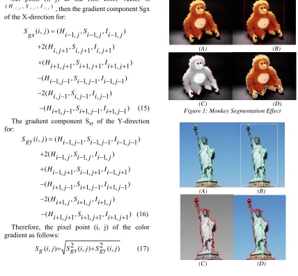
In order to verify the feasibility and effectiveness of the proposed method, we test related four group experiments. On Pentium dual-core 2.0G processor, we achieve our proposed algorithm with matlab7.0. Respectively test comparison on CV model and this article HIS color space-based level set segmentation algorithm. The results are shown in Figure 1 - Figure 4. (a) The original image, (b) Initial contour of the level set, (c) CV model segmentation effect, (d) the proposed method segmentation effect.

(A) (B)

[image:4.612.84.512.343.740.2]

(C) (D) Figure 1: Monkey Segmentation Effect

(A) (B)

(5)

555

Figure 2: The Statue Of Liberty Segmentation Effect

(a) (b)

(C) (D) Figure 3: Flower Segmentation Effect

(a) (b)

(C) (D)

Figure 4: Geometric Figure Segmentation Effect

From Figure 1 to Figure 4 can be seen, using the classic level set the CV model approach dividing the color image, especially in the close proximity of the target and the background gray, the part of the foreground object is mistakenly divided into the background, but also the background is mistakenly the case is divided into a foreground. Results using a text split, even if the current background gray near to prospects for a more precise segmentation, better color image segmentation.

Table I is the experimental comparison results for image segmentation. In Table I,segmentation times 1 is the number of iterations of the CV method corresponding level set, and segmentation times 2 is the number of iterations of the corresponding level set in the proposed method.T1 and T2, respectively are spent time for the CV method and the method we proposed. It is not difficult to see that the proposed method than CV method has greatly improved on the speed.

TABLE I : Table Comparison Results

Sample

CV method The proposed method

Segmentat-ion times 1

runnin g time

T1/s

Segmentat- ion times 2

runnin g time

T2/s

Figure 1

(350*262) 230 9.33 55 2.79

Figure 2

(323*400) 150 3.86 30 0.82

Figure 3

(375*248) 320 14.61 60 3.18

Figure 4

(256*256) 200 8.79 50 2.43

5 CONCLUSION

This paper presents a color image segmentation algorithm based on the level set of HIS color space. First, in order to improve the segmentation speed, we adopt fast level set method based on the CV model evolution. Secondly, for color images, we use the concept of the introduction of the color difference in the HIS color model space. Due to the full use of the color information of the image, considering the hue, saturation and intensity of the image, even if the color image gradation is close or the same, we still precisely segment image. The experimental results show that, compared with the conventional level set segmentation, our method for color images has better segmentation effect and it is faster.

REFRENCES:

[1] S. Osher, J. Sethian, “Fronts propagating with curvature dependent speed: Algorithms based on Hamilton-Jacobi formulations”, Comput. Phys. , vol. 79, no. 1, 1988,PP.12–49.

[2] F.T.Chan, L.Vese, “Active contours without edges”, IEEE Transactions on Image Processing, Vol. 10, No.2, 2001, pp.266-277. [3] Mumford D, Shah J, “Optimal approximation

by piece-wise smooth functions and associated variational problems”, Communications on Pure and Applied Mathematics, Vol. 42, No.5, 1989, pp.577-685.

[4] Shi Yongang, Karl William Clem, “A Real-Time Algorithm for the Approximation of Level-Set-Based Curve Evolution”, IEEE TRANSACTIONS ON IMAGE PROCESSING, Vol. 17, No.5, 2008, pp.645-656.

(6)

556 on Bayesian Classifier”,Proceedings International Conference on Computer Science and Software Engineering, IEEE Computer Society, December 12-14, 2008, pp.886-890. [6] Allili, Mohand Saïd, Ziou, Djemel, “An

automatic segmentation of color images by using a combination of mixture modelling and adaptive region information: A level set approach”, IEEE International Conference on Image Processing, IEEE, September 11-14, 2005, pp.305-308.

[7] LI Jun, YANG Xin, SHI Peng-Fei, “A Fast Level Set Approach to Image Segmentation Based on Mumford-Shah Model”, Chinese Journal of Computers, Vol. 25, No.11, 2002, pp.1175-1183.

[8] Osher S, Sethian J A, “Fronts propagating with curvature-dependent speed: Algorithms based on Hamilton-Jacobi formulations”, Journal of Computational Physics, Vol. 79, No.1, 1988, pp: 12-49.