Article
A Distributed Energy-Balanced Topology Control
Algorithm based on a Noncooperative Game for
Wireless Sensor Networks
Yongwen Du∗, Junhui Gong, Zhangmin Wang and Ning Xu
1
2
3
4
5
6
7
8
9
10
11
12
LanzhouJiaotongUniversity,TheSchoolofElectronics&InformationEngineering,Lanzhou730070,China; [email protected]
* Correspondence:[email protected]
Abstract:Inwirelesssensornetworks,thereisnoacentralcontrollertoenforcecooperationbetween nodes. Therefore,nodesmaygenerateselfishbehaviortoconservetheirenergyr esources.Inthis paper,weaddresstheproblemsoftransmissionpowerminimizationandenergybalanceinwireless sensor networks using a topology control algorithm. We consideredthe energy efficiencyand energybalanceofthenodes,andanimprovedoptimization-integratedutilityfunctionisdesignedby introducingtheTheilindex.Basedonthis,atopologicalcontrolgamemodelofenergybalanceis established,anditisprovedthatthetopologicalgamemodelisanordinalpotentialgamewithPareto optimality.Additionally,anenergy-balancedtopologycontrolgamealgorithm(EBTG)isproposedto constructtopologies.Thesimulationandcomparisonshowthat,comparedwithothertopological control algorithmsbasedongametheory,theEBTGalgorithmcanimproveenergybalanceand energyefficiencywhilereducingthetransmittingpowerofn odes,thusprolongingthenetwork lifetime.
Keywords:wirelesssensornetworks;topologycontrol;gametheory;energybalanced 13
1. Introduction 14
WSN (Wireless sensor networks, WSN) usually consist of a large number of sensor nodes. In 15
general, sensor nodes operate on batteries and are thus limited in their working lifetime [1]; therefore, 16
efficient and balanced energy usage is the key to prolonging the lifetime of a network, which is the 17
primary concern of topology control. The goal of topology control is to optimize the transmitting 18
power of each node and construct a better topology to improve network performance and prolong 19
network lifetime [2]. 20
At present, in the field of wireless sensor networks, many topological control algorithms, which 21
are mainly divided into hierarchical, power control, and game-type topology control algorithms, are 22
proposed. For example, a low-power hierarchical WSN topology control algorithm [3], which is a 23
multilevel topology control algorithm, is designed; this algorithm extends the network level and 24
improves the maintainability of WSN using a combination of the static address and the dynamic 25
address. In another paper [4], an energy-efficient hierarchical topology control method is established in 26
WSN using time slots, in which a cluster-head selecting approach decreases the difference in the cluster 27
size of LEACH and the responsibility mechanism for the active node makes the energy consumption 28
uniform in the cluster. In the literature [5], Kubisch et al. implement dynamic power control to set 29
the node degree of the upper and lower limits, thus resulting in a lower total energy consumption 30
network topology. The power control algorithm proposed in [6] uses a Borel Cayley graph to construct 31
a network topology that has a short average link and low energy consumption. The algorithm does 32
not consider the robustness of the network topology and the residual energy of nodes, which affects 33
the operation of the network to some extent. 34
When the sensor nodes perform data forwarding, the node will show selfish behavior due to 35
energy saving considerations, and competition will occur between nodes [7]. On this basis, the game 36
theory approach can be introduced into the study of WSN topology control. Game theory provides a 37
powerful tool [8] for describing the phenomena competition and individual coping strategies between 38
intelligent rational decision-makers, and it has been used in systems concerning action and payoff. 39
Komali et al. [9], [10] formulated energy-efficient topology control as a noncooperative potential game, 40
which guarantees the existence of at least one Nash equilibrium (NE) and proposes a distributed 41
noncooperative game topology control algorithm based on game theory. In [11], a topology control 42
algorithm based on a link power consumption game is designed to run the minimum MLPT algorithm 43
for the maximum power of the node. To consider network lifetime as well, researchers have proposed 44
two game-based topology control algorithms: the virtual game-based energy-balanced algorithm 45
(VGEB) [12] and the energy welfare topology control algorithm (EWTC) [13]; these algorithms have 46
been developed to improve network lifetime via energy-balanced network topologies. In [14], the 47
adaptive cooperative topological control algorithm (CTCA) based on game theory considers the 48
smallest potential lifetime and degree as the primary and secondary utility functions, respectively. 49
In [15], a topology control algorithm (DEBA) based on the ordinal potential game is proposed by 50
designing a payoff function that considers both network connectivity and the energy balance of nodes. 51
Although some of the abovementioned algorithms based on game theory can achieve network topology 52
control and improve network performance, they cannot guarantee the connectivity and robustness of 53
the network. Additionally, the remaining energy, energy balance and energy efficiency of the nodes 54
are not fully and accurately considered. 55
Based on the above analysis, this paper takes the energy efficiency and energy balance of the 56
node as the starting point and considers the influence of the residual energy, the transmitting power 57
and the node degree of the node. In addition, by introducing the Theil index to design an improved 58
and optimized integrated utility function, an energy-balanced topology control game algorithm 59
(EBTG) is proposed. The network topology constructed by this algorithm can efficiently guarantee the 60
connectivity and robustness of the network and balance the energy between nodes, which effectively 61
prolongs the network lifetime. 62
The rest of the paper is organized as follows. Section 2 overviews critical concepts of the network 63
model and the theory of potential games as applicable to our problem. Section 3 presents the topology 64
control game model and provides the game formulation and theoretic analysis. From this model, in 65
Section 4, an energy-balanced topology control algorithm, in which each sensor adaptively adjusts its 66
transmit power according to the residual energy, is proposed. Section 5 validates our EBTG algorithm 67
via simulation. Finally, Section 6 concludes this paper. 68
2. Preliminaries 69
In this section, we present a brief overview of some fundamental concepts related to the network 70
model, the ordinal potential game theory and the Theil index. 71
2.1. Network model 72
WSN are usually abstractedG= (N,L,P)as according to graph theory. LetG = (N,L,P)be an 73
undirected graph, whereNdenotes the set of nodes,Lis a set of two-node communication links in 74
node setNat timet, andPrepresents the transmit power set ofnnodes. 75
It is assumed that all nodes are randomly deployed in the plane monitoring area and that their 76
maximum transmit powerpmaxi can be different. When the transmit power pi ∈[0,pmaxi ]of nodeiis
77
sufficiently large, the signal received by nodejis higher than the receiving thresholdpso that nodej 78
Because most routing and channel studies use bidirectional links, it is assumed that the links in 80
the network topology are bidirectional. When all nodes use their maximum power to communicate, 81
the formed network topology is denoted byGmax. In this design,Gmaxis the connected network.
82
2.2. Ordinal potential game theory 83
The ordinal potential game is a kind of strategy game. The strategy gameΓconsists ofNplayers, the possible strategySof the players, and consequencesuof the strategy. The following definition is given for the strategy game:
Γ=hN,S,{ui}i (1)
Three definitions are as follows. First, (1)N={1, 2, 3,· · ·,n}represents the set of players, andnis the 84
number of players in the game. Then, (2)Srepresents the policy space, andSis the Cartesian product of 85
the set of policiesSi(i∈ N), whereSi={si1,si2,· · ·,sik}represents an optional set of policies for node
86
i, which is usually abbreviated asSi={s1,s2,· · ·,sk}. In general, we uses= (si,s−i)∈Sto describe
87
a strategy combination,sito represent the strategy choice of nodei, ands−ito represent the other node
88
strategy choices except nodei. Finally, (3)urepresents the utility functionu={u1,u2,· · ·,un}, where
89
uidenotes the maximum utility function that nodeican achieve in the policy combination(si,s−i).
90
Definition 1. In a strategy game Γ = hN,S,{ui}i, the strategy s∗i of any game player i is the best
91
strategy response to the strategy combination of s∗−i the remaining game participants. Then, there must 92
be uis1∗,· · ·,s∗i,· · ·,s∗n ≥ui n
s∗1,· · ·,s∗ij,· · ·,s∗no, where sijindicates that the j-th strategy of game player
93
i is valid for any sij∈S; then,
s∗1,· · ·,s∗n is called the "Nash Equilibrium (NE) [16]" of the game. 94
A game may possess a large amount of NEs or none at all, but some types of games have been 95
proved to have at least one Nash equilibrium, such as the ordinal potential game used in this paper, 96
which has been proved to be a Nash equilibrium and may not be unique in the literature [17]. 97
Definition 2. A strategic gameΓ=hN,S,{ui}iis an ordinal potential game if there exists a function V such
that∀i∈ N,∀s−i ∈S−iand for∀ai,bi∈S
V(ai,s−i)−V(bi,s−i)>0⇔ui(ai,s−i)−ui(bi,s−i)>0 (2)
The function V is called the ordinal potential function of the strategy gameΓ. Then, the strategy combination s∗ 98
for the maximum value of the ordinal potential function V is the NE of the game [17]. 99
2.3. Theil index 100
The Theil index [18] is a statistic primarily used to measure economic inequality and other economic phenomena. It was proposed by econometrician Henri Theil at Erasmus University in Rotterdam. This index measures income inequality through the concept of entropy in information theory [19]. When the concept of the entropy index in information theory is used to measure the income gap, the income gap can be interpreted as the amount of information contained in the message that converts the population share into the income share. The Theil indexTis defined as:
T= N
∑
i=1 xi
∑N
j=1xj
·lnxi x
!
(3)
wherexiis a characteristic of agenti,xrepresents average income, andNis the population. The range
101
3. Topology control game model 103
In this section, a topology control game model is first constructed. Then, it is proved that the 104
game model belongs to the ordinal potential game and the NE is Pareto optimal. 105
3.1. Utility function 106
The use environment of wireless sensor networks is relatively complex, and it is difficult to 107
quantify the benefits of nodes. The existing topology control algorithm based on the ordinal potential 108
game [15] does not adequately consider node revenue, and the utility function cannot accurately reflect 109
the competition between nodes and the balance of energy consumption. 110
This paper uses a power control model based on the utility function [17]. To maximize utility 111
function, each participant adjusts power in a selfish manner, which is typical for noncooperative power 112
control games. In addition, to better balance the load between nodes, energy efficiency is improved. In 113
this paper, the Theil index is introduced in the design of the utility function. In addition, the method of 114
measuring income inequality in the field of social science is used to measure the imbalance of energy 115
consumption between nodes in wireless sensor networks by using the node and its surplus energy as 116
analogues for the group members and their income. Thus, a more accurate node utility function is 117
obtained to describe the competitive relationship between nodes. 118
Consider a multihop network constituting independent and selfish nodes that adapt the transmit power levels according to their connectivity and energy consumption preferences. By considering the energy efficiency and energy balance, a specific utility function for nodei(∀i∈ N)is given by:
ui(pi,p−i) = fpi
λpmaxi −kpipi+ 1
T+1
+ Er(i)
E0(i)−Er(i)
+µEi(pi) (4)
where, for node i, initial energy, residual energy, current transmitting power and maximum transmitting power areE0(i),Er(i),piandpmaxi ,p−irepresents the transmit power of the remaining
n-1 nodes except nodei. In addition, we define a link state variable fpi fpi ≥0. If the network is
connected, then fpi =1; otherwise, fpi =0. Topology control aims to prolong the network lifetime
by reducing the node power without destroying the overall network connectivity and robustness. By adding parameter fpi fpi ≥0
, it is ensured that the network remains connected after repeated iterations of the game. Thekpirepresents the degree of nodeiwhen the transmitting power ispi;λand µare the weight factors of the utility function and all are positive numbers.Ei(pi) = m1
m ∑ j=1
Er(j)
E0(j)−Er(j)
(nodejmeans that nodeiis a single hop neighbor node at powerpi, wheremrepresents the number of
one-hop neighbor nodes of nodei) in equation4indicates that more calls to the remaining high-energy nodes participate in the communication link to ensure load balancing [11]. To better balance the load between nodes and improve energy efficiency, the method of measuring income inequality in the field of social science is used to measure the imbalance of energy consumption between nodes in wireless sensor networks using the node and its residual energy as an analogue for group members and their income; the Theil indexTis defined as
T= n
∑
i=1
Er(i) n ∑ j=1
Er(j)
·lnEr(i) Er
.
The utility function satisfies the properties described in [20]. With the utility function defined, a 119
3.2. Model proof 121
We show that the gameΓ=hN,S,{ui}iwith the utility function of each sensor given by (4) is an
122
ordinal potential game; then, the existence of NEs are guaranteed. 123
Theorem 1. The gameΓ=hN,S,{ui}iis an ordinal potential game. The ordinal potential function is given
by:
V(pi,p−i) =
∑
i∈N
fpi
λpmaxi −kpipi+
1 T+1
+ Er(i)
E0(i)−Er(i)
+µEi(pi)
(5)
Proof. We apply the asserted ordinal potential game in (4). First, we have:
∆ui =ui(pi,p−i)−ui(qi,p−i)
= fpi
λpmaxi −kpipi+
1 T+1
+µEi(pi)− fqi
λpmaxi −kpiqi+
1 T+1
−µEi(qi)
= fpi−fqi
λpmaxi + 1
T+1
+fqikqiqi− fpikpipi+µ
Ei(pi)−Ei(qi)
(6)
Similarly:
∆V=V(pi,p−i)−V(qi,p−i)
=
∑
i∈N
fpi
λpmaxi −kpipi+
1
T+1 +µEi(pi)
−
∑
i∈N
fqi
λpmaxi −kpiqi+
1
T+1+µEi(qi)
= fpi−fqi
λpmaxi + 1
T+1
+fqikqiqi−fpikpipi+µ
Ei(pi)−Ei(qi)
+
∑
j∈N,j6=i h
λ
fpj− fqj
pmaxj +µEj(pj) i
(7)
Thus, we have:
∆V=∆ui+
∑
j∈N,j6=i h
λ
fpj− fqj
pmaxj +µEj(pj) i
(8)
For nodei, because is monotonic andλ
fpj−fqj
pmaxj +µEj(pj)≥0, it follows from (6) that:
∆ui=
≥0 i f pi >qi and fpi > fqi
≤0 i f pi <qi and fpi < fqi
>0 i f pi >qi and fpi = fqi
<0 i f pi >qi and fpi = fqi
(9)
Therefore,sgn(∆ui) =sgn(∆V), the functionV(pi,p−i)is the ordinal potential function of the strategy
124
game, and the strategy gameΓ=hN,S,{ui}iis the ordinal game.
125
Theorem 2. The NE of the topology game model established in this paper is Pareto optimal [16] if the network 126
Gmaxis connected.
127
Proof. Due to the limited number of nodes, a node has a limited number of optional power 128
concentration elements. According to [17], the finite ordinal potential game must converge to the NE. 129
According to the definition of the network model and the description of the utility function, a node 130
the node continuously reduces the transmitting power and prolongs the survival time until the power 132
of all nodes no longer changes; that is, the NE state is reached. 133
When a NE point is reached, if a node reduces its power, network connectivity will be destroyed. 134
As a result, the remaining nodes must increase their power, thus resulting in lower utility function 135
values of other nodes and disruption of the NE. Therefore, according to the Pareto optimal definition, 136
it can be concluded that the NE of the topological control game is Pareto optimal. 137
4. Energy-balanced topology control game algorithm 138
In this section, we propose an energy-balanced topology control algorithm in which each sensor 139
adaptively adjusts its transmit power according to the residual energy. 140
Nodes in EBTG initiate with the maximum power networkGmax and then try to update this
141
topology iteratively according to their increasing unwillingness. EBTG consists of three phases: the 142
initialization phase (topological establishment phase), the adaptation phase (power adjustment phase), 143
and the topology maintenance phase. 144
4.1. Initialization phase 145
Every node in topology control game algorithms that makes a topological decision needs to collect 146
some network information. In EBTG, the information required by nodeiin the topology construction 147
process is the local topologyGi, which is an induced subgraph ofGmax. Every vertex of the directed
148
graph corresponds to a node in WSN. 149
To obtain this decision information, node i initializes its transmit power with maximum power 150
pmaxand discovers its neighbor nodes by broadcasting the "Hello" Message and collecting the responses
151
provided by the receivers atpmax. The message contains information such as node ID and remaining
152
energy. By receiving and returning the message, a series of information, such as ID, transmit power 153
and residual energy of its neighbor nodes, is learned and the maximum reachable neighbor setNmax(i)
154
of nodeiand its maximum uplink setLmax(i)is determined. By establishing these sets, the largest
155
global network topology viewGmaxcan be learned, thereby establishing a basis for subsequent routing
156
decisions. 157
4.2. Adaptation phase 158
Nodeiin the adaptation phase determines its transmit power according to its current residual 159
energyEr(i), the current transmitting power and the topology-related information collected during
160
Algorithm 1EBTG Power Adaptation initialization
1: nodeibroadcasts "hello" message atpimax 2: determine the neighbor setNmax(i)
3: Determine the optional power setPifor nodei, descending sort
4: Broadcast optional power setPi
Power adjustment
1: Pi={p1,p2,· · ·,pk}, descending sort
2: whilepiis not NE
3: fori=1,i≤N,i+ +
4: choose power according top∗i =arg max
pi∈Pi
ui(pi,p−i)
5: ifu∗i p∗i,p−i≥ui(pi,p−i)
6: ifpiis NE
7: pi =p∗i, updatepi
8: end if
9: end if
10: end for
11: broadcast a "hello" message including the new power settingpiatpmaxi
12: end while
This paper adjusts the network topology structure through the power control method, sets the 162
transmission power of the node as the optimal transmission power, and thus obtains the optimized 163
network topological structure. 164
In the power adaptation phase, we first need to sort the node’s strategy setPi ={p1,p2,· · ·,pk}
165
in descending order. The minimum available transmit powerpmini of nodeican be calculated using 166
the free-space model proposed in [21]. Pseudocode is shown in Algorithm1. 167
The power adjustment sequence of the EBTG algorithm is based on the node ID, as shown in 168
Fig. 1, the transmit power of one node is adjusted for each round, and the remaining power of 169
the node is unchanged. To ensure convergence to the NE, this algorithm uses the better response 170
strategy update scheme proved in [17], which converges to the NE in the finite ordinal potential game. 171
Given the powerp−iof other participants, the optimal response of nodeiisri(p−i) =min pmaxi ,p∗i,
172
which hasp∗i =arg max
pi∈Pi
ui(pi,p−i). During the game, when the node selects a power lower than the
173
current transmit power for communication, it is observed whether the corresponding integrated utility 174
function value increases. If it is larger, it indicates that the lower power is more suitable for use as the 175
Topology maintenance?
N
Y
Y
N
End Star
Update node power Broadcast to discover new
neighbors
Update network topology graph G
Set to transmit powerpi
i *
choose power according t argma ,
o x
i
i i i i
p P
p u p p
Pi is NE?
After initialization phase obtain the optional power set pi
,
Figure 1.Flowchart of Power Adaptation
When the power of the node is changed, the communication radius, the neighboring node and 177
its related links will change, which leads to the change of the network topology. As shown in Fig. 178
2, when the transmit power of nodeiincreases, nodejwill be included in its communication range; 179
then, the nearest neighbor node of nodeiis changed from the original nodekto the current nodej. 180
Therefore, nodejcan reduce its transmit power appropriately under the precondition of guaranteeing 181
full network connectivity. 182
i
k
j
T time coverage
T+1 time coverage
Figure 2.Diagram of Power Adaptation
4.3. Topology maintenance phase 183
As time flows, the energy consumption of the nodes may become more unbalanced. Therefore, 184
energy consumption between nodes will become unbalanced. In consideration of node failure or 185
phase, we designed an event-triggered approach that adaptively regenerates a more balanced network 187
topology. 188
The power game process can be implemented by comparing the residual energy of nodes with 189
the energy threshold or by setting the period to balance the load of nodes and prolong the network 190
lifetime. Pseudocode is shown in Algorithm2. 191
Algorithm 2EBTG Topology Maintenance initialization
1: Receiving neighbor information 2: ift≥T(Tis the set time threshold) 3: Replay the game of power adaptation 4: end if
Theorem 3. If theGmax is a connected network, the EBTG algorithm converges to the NE state that can
192
maintain the connectivity of networkGmax.
193
Proof. It is known from Theorem1that the topological control game model constructed in this paper is an ordinal potential game. In the EBTG algorithm proposed in this paper, the node increases its benefit function value by adjusting the choice of strategy (i.e., reducing the power value of the node) until the selection strategies of all nodes are not changed. Obviously, this state is a NE. It is assumed that the nodeiobtains greater benefits in the powerpi< p∗i, and the network is disconnected when
the powerp−iof the other nodes is unchanged; therefore:
ui(pi,p−i) = Er (i)
E0(i)−Er(i)
+µEi(pi)>λpmaxi −kpip ∗
i +
Er(i)
E0(i)−Er(i)
+µEi(p∗i) (10)
In addition, then:
µEi(pi)>λpmaxi −kpip ∗
i +µEi(p∗i) (11)
Obviously, equation (10) is not tenable, thus obtaining the connected network at each round of 194
the game execution of the EBTG algorithm. 195
5. Simulation results analysis 196
In this section, computer simulations are provided to illustrate the proposed algorithms. This 197
paper uses MATLAB R2016a as a simulation tool to simulate the EBTG algorithm. In addition, a 198
comparison with the DIA [10], MLPT [11] and DEBA [15] algorithms is conducted with regard to node 199
degree, node transmit power, node hop number and node residual energy. The experiment assumes 200
that all nodes are randomly deployed and cannot be moved, and each sensor sends a packet to other 201
sensors per second, i.e., each sensor transmits n-1 packets per second, the packet size is 1024 bytes, 202
and the transmission rate is 106 bits/s. The remaining emulation parameters are shown in Table1: 203
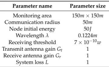
Table 1.Experimental parameter
Parameter name Parameter size
Monitoring area 150m×150m
Communication radius 50m
Node initial energy 50J
Wavelengthλ 0.1224m
Receiving threshold 7×10⁻¹⁰w
Transmit antenna gainGt 1
Receive antenna gainGr 1
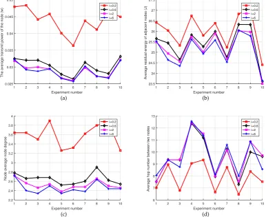
First, weight factorλandµin the utility function must be determined; the experiment randomly
204
distributes 50 nodes in the target region, as shown in Fig.3. 205
Forµ=1, the influence ofλon the network topology performance is considered in terms of the
206
average transmit power, the average node degree between nodes, the average residual energy of the 207
adjacent node and the average hop number of the shortest path between nodes. 208
Fig.3(a)indicates that the average transmit power of the node decreases asλincreases. Fig.3(b)
209
indicates that the residual energy of the neighboring node decreases asλincreases. Fig.3(c)indicates
210
that the average node degree of the network decreases asλ increases, but tends to stabilize after
211
λ≥2. Fig.3(d)indicates that the average hop number of the shortest path between nodes increases
212
asλincreases. The changes afterλ≥2 also tended to stabilize. From the general theory of network
213
topology, it can be seen that the topology of the network is perfect when the transmit power of the 214
nodes is low, while there is a moderate node degree and average hop number. By comprehensively 215
considering node computing power and network performance [22], this paper setsλ=4 andµ=1.
216
1 2 3 4 5 6 7 8 9 10
Experiment number 0.025
0.03 0.035 0.04 0.045 0.05
The average transmit power of the node (w)
λ=0.2
λ=0.6
λ=2
λ=6
(a)
1 2 3 4 5 6 7 8 9 10
Experiment number 23.5
24 24.5 25 25.5 26 26.5 27 27.5
Average residual energy of adjacent nodes (J)
λ=0.2
λ=0.6
λ=2
λ=6
(b)
1 2 3 4 5 6 7 8 9 10 Experiment number
2.2 2.4 2.6 2.8 3 3.2 3.4 3.6 3.8 4
Node average node degree
λ=0.2
λ=0.6
λ=2
λ=6
(c)
1 2 3 4 5 6 7 8 9 10
Experiment number 6
7 8 9 10 11 12 13
Average hop number between two nodes
λ=0.2 λ=0.6 λ=2 λ=6
(d)
Figure 3.The impact ofλon network performance
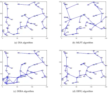
Fig.4shows the network topology diagram of the four algorithms, i.e., DIA, MLPT, DEBA and 217
EBTG. It can be seen that the network topology built by the DIA algorithm has a large load and low 218
residual energy (the nodes are marked out). The DEBA algorithm has a higher node degree and more 219
redundant nodes, which lead to faster energy consumption. Compared to the other two algorithms, 220
the MLPT and EBTG algorithms have lower node degrees and fewer redundant nodes. The general 221
theory of network topology shows that the EBTG algorithm has moderate nodes and redundant nodes; 222
therefore, its network connectivity and robustness are better than those of the other three algorithms, 223
0 50 100 150 0 50 100 150 28 27 30 16 23 24 19 22 28 25 22 20 18 17 18 21 34 24 25 30 31 22 23 24 25 22 30 21 23 23 25 20 16 22 24 30 14 25 28 27 31 28 22 31 29 25 23 33 30 23
(a) DIA algorithm
0 50 100 150
0 50 100 150 28 27 30 16 23 24 19 22 28 25 22 20 18 17 18 21 34 24 25 30 31 22 23 24 25 22 30 21 23 23 25 20 16 22 24 30 14 25 28 27 31 28 22 31 29 25 23 33 30 23
(b) MLPT algorithm
0 50 100 150
0 50 100 150 28 27 30 16 23 24 19 22 28 25 22 20 18 17 18 21 34 24 25 30 31 22 23 24 25 22 30 21 23 23 25 20 16 22 24 30 14 25 28 27 31 28 22 31 29 25 23 33 30 23
(c) DEBA algorithm
0 50 100 150
0 50 100 150 28 27 30 16 23 24 19 22 28 25 22 20 18 17 18 21 34 24 25 30 31 22 23 24 25 22 30 21 23 23 25 20 16 22 24 30 14 25 28 27 31 28 22 31 29 25 23 33 30 23
(d) EBTG algorithm
Figure 4.Network topology comparison chart
To make a clearer comparison of the four algorithms, this paper conducted 8 groups of 225
experiments. The specific experimental parameters are set as shown in Table1, where the number 226
of nodes participating in the experiment is increased from 30 to 100 and the algorithm is compared 227
by calculating the node transmit power of the four algorithms, the hops of the shortest link between 228
nodes and the average value of the four parameters of the node degree. 229
Fig. 5is a comparison diagram of the transmission power between nodes. It can be observed 230
from the figure that the transmission power of a node decreases as the number of nodes increases. The 231
EBTG algorithm’s node average transmit power is lower than the DIA, MLPT and DEBA algorithms, 232
which can ensure that the EBTG algorithm can establish network topology connections with lower 233
power, which is conducive to extending the network lifetime. 234
30 40 50 60 70 80 90 100 Number of nodes
0.005 0.01 0.015 0.02 0.025 0.03 0.035
Node average transmit power(w)
DIA MLPT DEBA EBTG
Fig.6shows the hop count comparison of the shortest link between nodes. The average hop count 235
of the EBTG algorithm is higher than that of the MLPT algorithm, but it is still lower than the DIA and 236
DEBA algorithms. The MLPT algorithm has higher node transmit power and greater communication 237
coverage, and so its average link hop count is lower. Since the EBTG algorithm operates at lower power 238
and the communication radius is smaller, the average hop count of the link increases. However, the 239
EBTG algorithm still obtains fewer link hops than the DIA and DEBA algorithms when the transmit 240
power is lower than the DIA algorithm. 241
30 40 50 60 70 80 90 100
Number of nodes 4
6 8 10 12 14 16
Average number of hops for the shortest link
DIA MLPT DEBA EBTG
Figure 6.Average number of hops for the shortest link
Fig.7shows a comparison of node degrees for the four algorithms. Because nodes with more 242
energy remaining in the EBTG algorithm are more active in node communication, to obtain a more 243
balanced load to prolong the life cycle of the network, the node degree is higher than that of the 244
DIA algorithm but lower than that of the DEBA and MLPT algorithms. The moderate node degree 245
of the EBTG algorithm does occupy too much of the energy resources and obtains relatively good 246
connectivity and robustness, while having fewer redundant nodes can achieve better energy efficiency, 247
improve channel multiplexing and reduce interference. 248
30 40 50 60 70 80 90 100
Number of nodes 1.5
2 2.5 3 3.5 4
Average node degree
DIA MLPT DEBA EBTG
Figure 7.Average node degree
Fig. 8compares the standard deviations of the node residual energy. It can be seen that the 249
variance of the EBTG algorithm changes slowly. In the network topology constructed by the DIA, 250
MLPT, and DEBA algorithms, the load of some nodes is too high, which affects the network lifetime. If 251
these heavily loaded nodes die prematurely, they will also have a greater impact on the connectivity and 252
robustness of the network. The DIA algorithm overemphasizes that reducing the node transmit power 253
makes the network energy consumption uneven; the MLPT algorithm does not consider the node’s 254
residual energy, resulting in poor performance of its energy balance; the DEBA algorithm focuses on 255
energy balance while ignoring the energy efficiency, which leads to the growth of the residual energy 256
not only considers the remaining energy of the node but also transfers the data forwarding task to 258
nodes with more residual energy, effectively balancing the load of the entire network and improving 259
energy efficiency. 260
0 10 20 30 40 50 60 70 80 90 100 4.5
5 5.5 6 6.5 7 7.5 8 8.5 9
Standard deviation of remaining energy
DIA MLPT DEBA EBTG
Figure 8.Standard deviation of node residual energy
Fig.9is a network lifetime comparison chart. Because topology control is mainly concerned with 261
energy, prolonging the network life cycle is an important index for evaluating the topology control 262
algorithm. The graph shows that the network lifetime of the EBTG algorithm is the longest because 263
the EBTG algorithm reduces the transmit power of the node, expertly balances the load between nodes 264
and improves the energy efficiency; therefore, its network lifetime is much higher than that of the 265
networks constructed using the DIA, MLPT and DEBA algorithms. 266
DIA MLPT DEBA EBTG
Algorithm type 0
1 2 3 4 5 6 7×10⁴
Figure 9.Network lifetime
6. Conclusions 267
Sensors in wireless sensor networks have been restricted to local communications and make 268
topological decisions selfishly, and the unbalanced energy consumption between nodes is likely to 269
shorten the network lifetime. 270
Based on the theory of potential games and the Theil index, this paper designs an optimized 271
utility function that considers the residual energy of nodes, the transmitting power of nodes and the 272
connectivity of the network. On this basis, a topological game model is constructed. Additionally, it 273
is proved that a Pareto-optimal NE exists in this model. Thus, an energy-balanced WSN distributed 274
topology game algorithm called EBTG is proposed. From the simulation results, it can be concluded 275
that the EBTG algorithm can effectively reduce the power of the transmitting node, balance the load 276
between nodes, improve the energy efficiency of the network and prolong the network lifetime to 277
this algorithm in the real-world wireless communication environment to improve the reliability and 279
stability of the algorithm. 280
Author Contributions:Conceptualization—Y.D. and J.G.; software—Y.D.; supervision—Y.D.; validation—N.X.;
281
writing (original draft)—Y.D.; writing, review, and editing—Z.W.
282
Funding: This work is partially supported by the National Natural Science Foundation of China (11461038,
283
61163009); Natural Science Foundation of Gansu Province(144NKCA040).
284
Conflicts of Interest:The authors declare no conflict of interest.
285
References 286
1. Yick, Jennifer, Biswanath Mukherjee, and Dipak Ghosal. "Wireless sensor network survey." Computer
287
networks 52.12 (2008): 2292-2330.
288
2. Ishmanov, Farruh, A. S. Malik, and S. W. Kim. "Energy consumption balancing (ECB) issues and
289
mechanisms in wireless sensor networks (WSNs): a comprehensive overview." European Transactions
290
on Telecommunications 22.4(2011):151–167.
291
3. Kang, Yi Mei, et al. "A Low-power Hierarchical Wireless Sensor Network Topology Control Algorithm."
292
Acta Automatica Sinica 36.4(2010):543-549.
293
4. Xiong, Shu Ming, L. M. Wang, and J. Y. Wu. "Energy-efficient hierarchical topology control in wireless sensor
294
networks using time slots." International Conference on Machine Learning and Cybernetics IEEE, 2008:33-39.
295
5. Kubisch, M., et al. "Distributed algorithms for transmission power control in wireless sensor networks."
296
Wireless Communications and Networking, 2003. WCNC 2003 IEEE, 2003:558-563 vol.1.
297
6. Yu, Jaewook, E. Noel, and K. W. Tang. "Degree Constrained Topology Control for Very Dense Wireless
298
Sensor Networks." Global Telecommunications Conference IEEE, 2011:1-6.
299
7. Charilas, Dimitris E. "A survey on game theory applications in wireless networks." Computer Networks
300
54.18(2010):3421-3430.
301
8. Mackenzie, A, and L. Dasilva. "Game theory for wireless engineers." Synthesis Lectures on Communications
302
1(2006):1-86.
303
9. Komali, Ramakant S, and A. B. Mackenzie. "Distributed topology control in ad-hoc networks: a game
304
theoretic perspective." Consumer Communications and NETWORKING Conference, 2006. Ccnc IEEE,
305
2006:563-568.
306
10. Komali, Ramakant S., A. B. Mackenzie, and R. P. Gilles. "Effect of Selfish Node Behavior on Efficient Topology
307
Design." IEEE Transactions on Mobile Computing 7.9(2008):1057-1070.
308
11. Zarifzadeh, Sajjad, N. Yazdani, and A. Nayyeri. "Energy-efficient topology control in wireless ad hoc
309
networks with selfish nodes." Computer Networks 56.2(2012):902-914.
310
12. Hao, Xiao Chen, et al. "Virtual Game-Based Energy Balanced Topology Control Algorithm for Wireless
311
Sensor Networks." Wireless Personal Communications 69.4(2013):1289-1308.
312
13. Abbasi, Mohammadjavad, and N. Fisal. "Noncooperative Game-Based Energy Welfare Topology Control for
313
Wireless Sensor Networks." IEEE Sensors Journal 15.4(2015):2344-2355.
314
14. Chu, Xiaoyu, and H. Sethu. "Cooperative Topology Control with Adaptation for improved lifetime in
315
wireless sensor networks." Ad Hoc Networks 30.C(2015):99-114.
316
15. Li, Xiao Long, D. L. Feng, and P. C. Peng. "A potential game based topology control algorithm for wireless
317
sensor networks." Acta Physica Sinica (2016).
318
16. Leiniger, Wolfgang. "Games and information: An introduction to game theory." International Journal of
319
Industrial Organization 9.3(1991):474-476.
320
17. Monderer, Dov, and L. S. Shapley. "Potential Games." Games & Economic Behavior 14.1(1996):124-143.
321
18. Silver W E. Economics and Information Theory[J]. Journal of the Operational Research Society, 1967,
322
18(3):328-328.
323
19. Theil, Henri. "Studies in Global Econometrics." Advanced Studies in Theoretical & Applied Econometrics
324
79.2(1996).
325
20. Shah, Viral, N. B. Mandayam, and D. J. Goodman. "Power control for wireless data based on utility and
326
pricing." IEEE International Symposium on Personal, Indoor and Mobile Radio Communications IEEE,
327
1998:1427-1432 vol.3.
21. Wang, Xijun, et al. "RESP: A k-connected residual energy-aware topology control algorithm for ad hoc
329
networks." Wireless Communications and NETWORKING Conference IEEE, 2013:1009-1014.
330
22. Ok, Changsoo, et al. "Distributed routing in wireless sensor networks using energy welfare metric."
331
Information Sciences 180.9(2010):1656-1670.