Brain response pattern identification of fMRI data using a particle
swarm optimization-based approach
Xinpei Ma.Chun-An Chou.Hiroki Sayama. Wanpracha Art Chaovalitwongse
Received: 31 October 2015 / Accepted: 15 March 2016 / Published online: 7 April 2016 ÓThe Author(s) 2016. This article is published with open access at Springerlink.com
Abstract Many neuroscience studies have been devoted to understand brain neural responses correlating to cogni-tion using funccogni-tional magnetic resonance imaging (fMRI). In contrast to univariate analysis to identify response pat-terns, it is shown that multi-voxel pattern analysis (MVPA) of fMRI data becomes a relatively effective approach using machine learning techniques in the recent literature. MVPA can be considered as a multi-objective pattern classification problem with the aim to optimize response patterns, in which informative voxels interacting with each other are selected, achieving high classification accuracy associated with cognitive stimulus conditions. To solve the problem, we propose a feature interaction detection framework, integrating hierarchical heterogeneous particle swarm optimization and support vector machines, for voxel selection in MVPA. In the proposed approach, we first select the most informative voxels and then identify a
response pattern based on the connectivity of the selected voxels. The effectiveness of the proposed approach was examined for the Haxby’s dataset of object-level repre-sentations. The computational results demonstrated higher classification accuracy by the extracted response patterns, compared to state-of-the-art feature selection algorithms, such as forward selection and backward selection.
Keywords Brain response pattern Brain functional connectivity Pattern classificationParticle swarm optimizationFeature selection Interaction selection
1 Introduction
Functional magnetic resonance imaging (fMRI) is one of the publicly used neuroimaging techniques to capture brain neural activity in small volumetric units (called voxels) in the brain by measuring the change of blood-oxygen-level dependent (BOLD) signals over time. Broadly speaking, it has advanced the understanding of brain functional activity by fMRI in various cognitive and behavioral neuroscience applications, such as Alzheimer’s disease [1], aging [2], autism [3], depression [4], schizophrenia [5], and attention-deficit hyperactivity disorder [6]. The overarching goal of these research studies with fMRI is to examine and understand the brain states among different regions of interest (ROI) associated with specific brain functions or disorders, so that treatments and interventions can be made precisely according to stimulus or diagnostic conditions [7].
Conventionally, univariate analysis of fMRI data was widely used to identify the ROIs of brain functions (i.e., localization) by statistical tests on individual voxels in most research studies [8,9]. In more recent years, multi-X. MaC.-A. Chou (&)H. Sayama
Department of Systems Science & Industrial Engineering, Binghamton University, the State University of New York, Binghamton, USA
e-mail: [email protected]
X. Ma
e-mail: [email protected]
H. Sayama
e-mail: [email protected]
W. A. Chaovalitwongse
Departments of Industrial & Systems Engineering, Department of Radiology, Integrated Brain Imaging Center, University of Washington, Seattle, USA
e-mail: [email protected]
W. A. Chaovalitwongse
Department of Radiology, Integrated Brain Imaging Center, University of Washington, Seattle, USA
voxel pattern analysis (MVPA) of fMRI data has been increasingly applied to identify response patterns of voxels as a whole [3, 10, 11]. The MVPA can be modeled as a high-dimensional pattern classification problem to train a classification (or prediction) model based on the fMRI BOLD signals, in which voxels (as features) are identified in response to stimulus or diagnostic conditions (as class labels). In most neuroscience experimental studies, the number of stimulus samples is relatively much less than the number of voxels in the brain. This leads to a computa-tional challenge of high feature-to-sample ratio from the machine learning viewpoint [12]. Therefore, various advanced feature selection and sparse optimization tech-niques were proposed to enhance the computational results in terms of classification efficacy and informativeness of selected voxels [13–17]. It leads to two-fold objectives: (1) it aims to select a minimum number of voxels included in classification models and (2) the classification accuracy needs to be maximized.
Technically, a number of computational approaches have been proposed and employed to solve this multi-ob-jective high-dimensional problem [18–21]. Computational intelligence-based approaches, such as genetic algorithms (GA), simulated annealing (SA), ant colony optimization (ACO), and particle swarm optimization (PSO), are at the forefront of this research [22–26]. They are implemented in conjunction with a classifier to find a set of highly repre-sentative features for classification tasks. Heuristic feature selection approaches stand out in terms of theoretical simplicity, strong global search ability, and less expensive computational cost. Instead of exhaustively exploring the solution space, these algorithms adopt effective learning schemes to optimize the feature selection [27]. In addition, heuristic approaches pay more attention to find the best combination of features rather than evaluating the good-ness of features individually. These benefits of computa-tional intelligence approaches indicate a great potential in analyzing brain response patterns of high-dimensional fMRI data [28].
However, when solving high-dimensional optimization problems where multiple local optima exist, most classical heuristic optimization algorithms fail to find (near) global optimal results. Limited by simple searching behaviors and communication abilities, classical heuristic optimization algorithms are easily stuck to local minima and therefore stop searching for better solutions in the problem space [29]. This phenomenon is referred to as premature con-vergence, which either leads to poor classification perfor-mance or results in the discovery of poor quality feature subsets [30]. Hierarchical heterogeneous particle swarm optimization (HHPSO), as a recently developed variation
problems by performing diverse searching behaviors [31]. As the success of HHPSO has demonstrated its strength in addressing high-dimensional and complex optimization problems, in this paper, we combine HHPSO with a linear support vector machine (HHPSO-SVM) to perform feature subset selection and classification tasks.
In this paper, extracting discriminating voxel-based brain response patterns that distinguish different cognitive states is a major goal. In MVPA of fMRI data, functional connectivity between individual voxels plays a pivotal role in distinguishing different cognitive states because they capture temporal dependency or causality between differ-ent brain regions [15, 17]. However, in existing fMRI analysis, functional connectivity patterns are not inten-sively analyzed as a whole due to an exponential increase in size of the search space. For this purpose, we develop a new feature interaction detection framework (FIDF) that focuses on identifying informative voxels and voxel-based functional connectivity in two sequential stages. The pro-posed HHPSO–SVM feature selection approach is imple-mented in this framework, which is first used to select informative voxels and then used to select a connectivity pattern. The well-known Haxby’s dataset [32] is used to evaluate the effectiveness of the proposed approach.
The rest of this paper is structured as follows. In Sect.2, the MVPA concept of fMRI data is presented with an explanation of the Haxby’s dataset. In Sect. 3, PSO and HHPSO with their applications are introduced. In Sect.4, the FIDF using a HHPSO–SVM feature selection algorithm is proposed. Experimental results are presented in Sect.5. In Sect. 6, this work is concluded with discussions and future work.
2 Multi-voxel pattern analysis of fMRI data
MVPA studies for cognitive state decoding by using fMRI are implemented in three steps: feature extraction, feature selection, and classification [13]. fMRI data for task-based analysis is a plethora of noisy time series measurements. It is usually important to filter out the noise and extract the useful information from this bulky data. In the feature extraction step, voxel responses for each stim-ulus conditions are mapped onto predefined standard hemodynamic response functions (HRF) and estimated the similarity indexes. This is achieved usually with two ways which are taking the average of the response across time to each stimulus condition and fitting a general linear model (GLM) to a standard hemodynamic response function (HRF) [38]. GLM provides a more representative value about the response of a voxel to the stimulus condition [39].
Feature (voxel) selection plays a vital role in MVPA. In this step, we aim to select a subset of informative voxels features in order to enhance the classification accuracy and/ or provide to neuroscientists more refined characteristics of brain functional responses. This task can be done according the predefined region of interest (ROI) identification based on the anatomical structure information in the brain [32]. Or it aims to choose voxels that are significantly active to stimuli by using univariate statistical tools such as ANOVA ort-test [40]. In addition, to score voxels according to their individual accuracy level in the experimental settings [40], mutual information [41] and partial least square regression [13] were also used for feature ranking and selection in the literature. Other than these univariate measures, recursive feature elimination is also applied as a multivariate tech-nique to select voxels [10], but the interactions among voxels are not clear yet. Searchlight accuracy based on the neighboring voxels’ contribution to classification for selecting the voxels is also a multivariate technique that considers spatial closeness of the voxels [40]. To the best of our knowledge, the interactions among the voxel activities have not been fully investigated yet in MVPA.
2.1 Haxby’s experiment of visual function
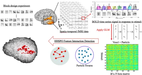
In this study, we use a benchmark dataset (of six subjects) experimented by Haxby’s research group for experimental tests [32]. In Haxby’s block-design experiment, each sub-ject contains 12 fMRI runs; in each run, eight stimulus blocks, each displaying image exemplars from a different conceptual category were displayed to the subject in a random order, as described in Fig.1(upper left). The fMRI data were collected from a GE 3T scanner. One image of brain activity in the dataset (consisting of 64 64 40 voxels) was acquired every repetition time (TR) of 2.5 seconds. Thus, there are a total of 9 TRs (=22.5/2.5) in each
block, yielding 720 data instances for the dataset (12 runs
8 blocks9 TRs). In our study, we only focused on the predetermined region (region of interest, ROI) of thresh-olded voxels with task-related variance in the ventral temporal cortex, as opposed to the whole-brain space (around 20,000–40,000 voxels).
To characterize the temporally evolving BOLD signal change in response to a stimulus, a general linear model (GLM) is applied, and coefficient parameters b are esti-mated by fitting a GLM with different predictors for each stimulus block. In this study, the predictors (i.e., si1;si2;. . .;siT for stimulus conditioni= 1 to 8, and BOLD
responses at time 1 to T) were modeled with a boxcar convolved with a canonical HRF [42]. We used a double-Gamma function provided by SPM [43], with the default settings, as the HRF. The b weights (parameters) are extracted for each run of the experiment, each generating a 3-dimensional bweight matrix for each voxel, which can be in turn transformed to a 2-dimensional feature matrix. We denote this input feature matrix F, whose size is MN, whereMis the number of data instances (the total number of presented stimuli) and Nis the number of fea-tures (voxels). The element fdj of the data matrixF
repre-sents the real-valued coefficient parameter b of the d-th data instance at thej-th voxel. It is helpful to viewfdjas the d-th sample of thej-th feature random variableFj, thej-th
column ofF. It is more convenient to treatFjas a random
variable of the real-valued coefficient b in relevant prob-abilistic measures. We denote class label ci2 f1;. . .;Kg
(i.e., stimulus category), where K is the total number of stimulus categories. For each data instance i,ci is known
precisely according to the experiment design. Figure 1
illustrates the framework to extract features from fMRI signals in the ventral temporal cortex in this case.
3 Hierarchical heterogeneous particle swarm optimization
3.1 PSO
Vit;þj1¼Vit;jxþc1r1t;i;j y^ t
jx
t i;j
þc2r2t;i;j y t i;jx
t i;j
ð1Þ
and
xtiþ;j1 ¼xti;jþVit;þj1; ð2Þ
whereVt
i;jdenotes the velocity of particleiat timet,x t i;j is
the particlei’scurrent position at timet,yt
i;jis the personal
best solution of particleiat time t, andy^t
jis the global best
solution obtained at timet. Subscriptjis the index of the spatial dimension.x is a parameter called inertia weight representing how much the particle’s memory can influ-ence the new position. c1 and c2 are two constant
accel-eration coefficients and rt
1;i;j and r2t;i;j are two random
numbers. They are used to balance exploration and exploitation search behaviors.
3.2 HHPSO
Even though the algorithm design of PSO is simple and computationally efficient, standard PSO is easily trapped into local minima, especially when the optimization problem is complex. In recent years, many variations of PSO have been proposed to overcome this premature convergence problem.
We have recently proposed HHPSO [31]. Compared to standard PSO, the swarm is equipped with multiple equally sized layers. During the search, particles dynam-ically arrange themselves in a hierarchical structure based on their current fitness values. The better the fitness is, the higher the position in the hierarchical structure is. In HHPSO, particles are not only attracted toward their personal best and global best positions, but they are also attracted toward attractors. For particles in the top layer, their attractors are particles in the same layers with better fitness. For the rest of particles (not in the top layer), their attractors are particles in their immediate superior layer. Herein, a particle’s new velocity is a cumulative effect of (a) its previous velocity, (b) its personal best position, (c) the global best position, and (d) positions of its attractor, as shown in Eq. (3).
Vit;þj1¼Vit;jxþc1rt1;i;j y^ t
jx
t i;j
þc2rt2;i;j y t i;jx
t i;j
þP
At i
a¼1
c3r3t;i;j xðiÞ t a;jx
t i;j
;
ð3Þ
wherexðiÞta;jis the position of attractor particleaof particle iin dimensionjat timet.At
iis the total number of attractors
of particlei at timet. c3 is a constant acceleration
coeffi-Fig. 1 An illustration of the proposed approach to response pattern
identification from which a block-design experiment is carried out to examine visual function of fMRI data. Representative features are extracted by applying GLM to BOLD time series across all voxels in
cient andrt
3;i;j is a random number. Other parameters are
exactly the same as those used in Eq. (1).
For the searching behavior, in HHPSO algorithm, parti-cles are allowed to perform different searching behaviors based on their ranks in the hierarchy and their current per-formances. For example, if a signal of premature conver-gence (i.e., early stagnation or overcrowding) is detected, the relevant particle will change its previously adopted search-ing behavior and randomly select a new searchsearch-ing behavior from the predefined behavior pool to avoid premature con-vergence [31]. Compared to standard PSO, HHPSO is more resistant to local minima and superior to sustain the popu-lation diversity as the dimension of the search space grows. Recently, PSO as well as its variations has been implemented as efficient global optimization techniques, which received considerable attention in machine learning (ML), data mining, and pattern recognition [46–48]. These algorithms have shown to perform very well on algorithm development and parameter optimization tasks [49–52].
4 HHPSO–SVM for voxel selection in MVPA
4.1 Problem definition
HHPSO–SVM feature selection algorithm (HHPSO–SVM) aims to maximize classification accuracy (Max-Accuracy) and to minimize the size of selected features (Min-Size) simultaneously. The objective function in Eq. (5), which is utilized to quantify searched solutions, is defined by dividing the classification error by the number of elimi-nated features. The penalization term (i.e., Min-Size) is used for the purpose of constructing a compact set of features and controlling overfitting. The approach iterates until a best solution (a subset of features) is found.
f ¼maxAccuracyðSiÞ
minSizeðSiÞ
ð4Þ
fi¼
ErrorðSiÞ NSizeðSiÞ
ð5Þ
In Eqs. (4) and (5),Sirepresents the feature subset selected
by particle i. AccuracyðSiÞ and ErrorðSiÞ represent the
classification accuracy and error calculated by using fea-ture subseti. N is the entire number of features. SizeðSiÞ
represents the number of features in subseti.
4.2 Algorithm design
In the HHPSO–SVM feature selection algorithm, HHPSO provides multiple candidate solutions to feature selection and SVM is employed to evaluate the classification per-formance using these candidate solutions. Particles
cooperate to locate a best solution in an N dimensional problem space, where N is the cardinality of the original feature set. Positions of particles are represented as numeric strings of length N. Each value in the string is within zero and one, which can be seen as the contribution of the corresponding feature to the classification task. The higher the value, the more important it is. Each particle selects a set of important features based on its position string.
Each iteration involves two steps (see Algorithm 1). In the first step, we identify the selected features and evaluate the fitness value for each particle (lines 1–10). Taking particlei for an example, a predefined threshold h is applied to its current positionxi. Thej-th feature will be selected, if thej-th
value in the position string is greater thanh. With the selected features, classification error as well as the number of elimi-nated features is calculated by SVM to evaluate the fitness value for particle i (see Eq. 5). After all particles finish updating their fitness values and their personal best solutions, the global best solution is defined by the best of the personal best solutions in the swarm.
In the second step, particles are ranked by their fitness values in an ascending order and directed to the right layer in the hierarchical structure (lines 11–15). Based on the rank, particles occupy layers from top to bottom. Particles in the higher layers always have better fitness values than particles in the lower layers.
In the third step, particles update their velocities and positions based on their searching performances as well as their positions in the hierarchical structure (lines 16–25). This step ensures that the swarm continuously explores the problem space and optimizes solutions iteration by iteration. The algorithm terminates when it converges to a sta-tionary solution, which is defined by a condition that the global best position stops to evolve for more than 50 iter-ations. As the algorithm converges, the final solution to feature selection is obtained by applying the threshold (h) to the global best position (line 26).
In HHPSO–SVM (Algorithm 1),Prepresents the swarm population, andPi represents particlei.nis the number of
particles in the swarm.Nis the dimension of the problem space.xi;jis particlei’s current position in dimensionj.Si
denotes the subset of features selected byPi.Fj represents
the j-th feature in the original feature space. yi represents
the personal best position of particleiat timet.y^represents the global best position.frepresents the fitness function.Ri
represents the i-th particle in the swarm, after sorting all particles by their fitness values in an ascending order. Lo
represents the first layer and Lj represents the ðjþ1Þ-th
layer.l andkare the number of layers and the number of particles in a layer, respectively. Ai denotes the set of
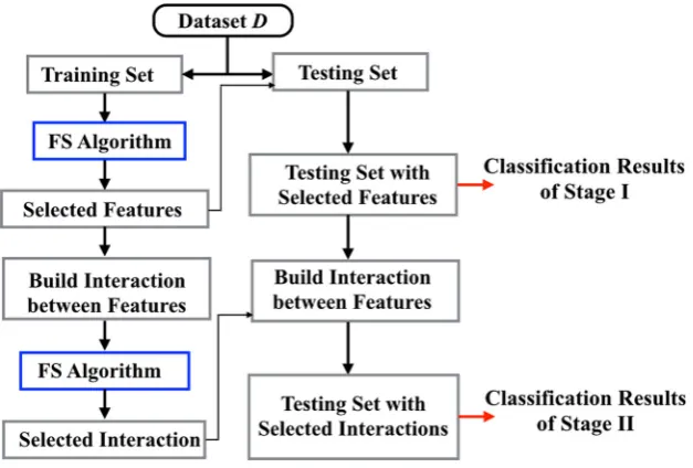
4.3 Feature interaction detection framework
In order to extract discriminating multi-voxel patterns from fMRI data, scalable, robust, and efficient dimension reduction tools are desired to identify influential voxels and voxel-based connectivity. In this paper, FIDF is developed as a MVPA approach that undergoes a two-stage
procedure. Voxel selection (feature selection) and voxel connectivity selection (feature interaction selection) are performed in Stage I and Stage II, separately. The proposed HHPSO–SVM is adopted as the feature selection method under this framework.
In the first stage, the feature selection algorithm is implemented to select the best subset of voxels. This procedure is repeated 15 times to obtain the average number of selected voxels (Navg) and frequencies of
voxels being selected. Voxels are ranked according to their selection frequencies in a descending order. The top N1 (N1 ¼ 1:05Navg) voxels are selected in Stage I. In the
second stage, we first establish all connectivity that con-nects voxels selected in Stage I, which is equivalent to constructing a fully connected network. In this stage, we aim at extracting discriminating connectivity patterns from a fully connected structure. The rationale is as fol-lows: HHPSO–SVM selects a best combination of voxels in the first stage, which means the selected voxels are interactive and informative as a combination. Identifying consistent connectivity patterns from the pre-selected voxel combination may achieve similar or even better classification performances than only considering indi-vidual voxels.
For fMRI data, the connectivity between two voxels is generated via finding products of all pairs of voxels. This type of connectivity definition is similar to using correla-tion coefficients, mutual informacorrela-tion, or consistency mea-sures to quantify the connectivity between two voxels. By doing this, the dimension of feature space becomes N1ðN11Þ=2. HHPSO–SVM is implemented again to
select the best subset of connectivity that distinguishes multiple classes. Similarly, this algorithm is repeated 15 times to identify robust connectivity patterns.
Fig. 2 A conceptual
In the present study, we utilize a 12-fold cross-valida-tion to assess the performance of different feature seleccross-valida-tion algorithms. We first divide the whole data into 12 portions of equal size. The optimization procedure is performed on the 11 portions of data, and the remaining 1 fold is held out to evaluate the algorithm’s performance. During opti-mization, the training set is further randomly split, in which 6 portions are used to train the model and the other 5 portions are used to test the results. The random splitting is repeated 20 times, and the average classification error rate and the average number of selected feature subsets are used to estimate the fitness function.
The final decision of feature selection is determined by the global best solution obtained at the end of optimization. The same threshold (h) and mechanism are applied to select a robust set of connectivity features. The classifica-tion performance is examined on the holdout dataset. Means and standard deviations are computed using this 12-fold cross-validation approach.
5 Experimental analysis
5.1 Experimental setting
Comparative experiments were carried out for the Haxby’s dataset [32]. For a comparison purpose, the same data preprocessing techniques, including using z-score to stan-dardize the data and randomly shuffling the original data matrix, were applied to attenuate noise and improve spatial alignment of time series data [53].
The performance of the proposed HHPSO–SVM selec-tion algorithm was evaluated by comparing it with (a) without feature selection (WFS), (b) sequential forward feature selection (SFS), (c) sequential backward feature selection (SBS), and (d) standard PSO feature selection algorithm (PSO–SVM). SFS and SBS are deterministic greedy algorithms and can only produce a single solution for each dataset. PSO–SVM combines standard PSO and linear SVM, and it adopts the same objective function to explore the best solution to feature selection. The mecha-nism of PSO–SVM is similar to HHPSO–SVM. All five algorithms were applied to FIDF to select voxels in the first stage and select voxel-based connectivity in the second stage.
In this study, both HHPSO–SVM and PSO–SVM employed a swarm containing 50 particles. The accelera-tion coefficients,c1andc2, are linearly changed over time.
c1 linearly decreased from 2.5 to 0.5, and c2 linearly
increased from 0.5 to 2.5 using the formula shown in Eqs. (6) and (7), wherentis the overall iteration time, andt
is the current iteration, as follows:
c1ðtÞ ¼ ðc1;minc1;maxÞ
t nt
þc1;max ð6Þ
and
Table 1 Classification results of Stage I of FIDF
Stage I WFS SFS SBS PSO–SVM HHPSO–SVM
Mean SD Mean SD Mean SD Mean SD Mean SD
Sbj 1 0.875 0.191 0.693 0.153 0.875 0.190 0.819 0.130 0.885 0.099
Sbj 2 0.708 0.106 0.517 0.140 0.708 0.106 0.623 0.141 0.696 0.143
Sbj 3 0.864 0.148 0.686 0.161 0.865 0.148 0.792 0.140 0.874 0.118
Sbj 4 0.677 0.148 0.560 0.150 0.677 0.148 0.676 0.155 0.708 0.186
Sbj 5 0.705 0.312 0.568 0.202 0.685 0.323 0.562 0.270 0.614 0.270
Sbj 6 0.875 0.125 0.684 0.180 0.875 0.125 0.805 0.122 0.852 0.104
The classification accuracy and standard deviations ofWFSwithout feature selection,SFSsequential forward feature selection,SBSsequential backward feature selection,PSO–SVMandHHPSO–SVMwere calculated for subject 1 to subject 6
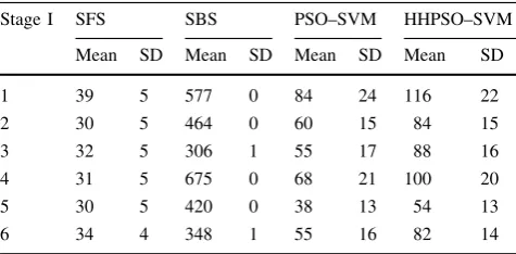
Table 2 The number of selected voxels in Stage I of FIDF
Stage I SFS SBS PSO–SVM HHPSO–SVM
Mean SD Mean SD Mean SD Mean SD
1 39 5 577 0 84 24 116 22
2 30 5 464 0 60 15 84 15
3 32 5 306 1 55 17 88 16
4 31 5 675 0 68 21 100 20
5 30 5 420 0 38 13 54 13
6 34 4 348 1 55 16 82 14
c2ðtÞ ¼ ðc2;maxc2;minÞ
t nt
þc2;min: ð7Þ
We implemented the linear support vector machine (SVM) from the scikit-learn in Python, with the parametercset to 1 in all experiments [54]. For both PSO and HHPSO, the value of threshold (h) is 0.95. For HHPSO, the hierarchical population structure consisted of five layers as shown in Fig.2.
5.2 Experimental results
The comparative classification results of the five different algorithms are summarized in Tables 1 (Stage I) and 3
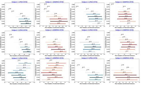
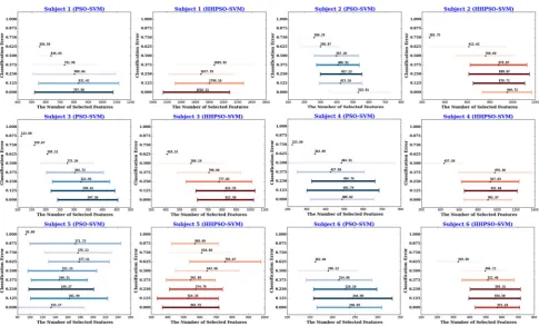
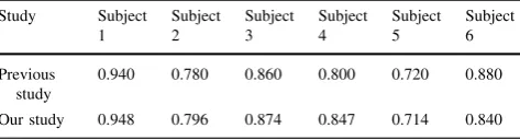
(Stage II). The statistics of the number of selected features are presented in Tables2 and 4 for Stage I and Stage II, respectively. For PSO–SVM and HHPSO–SVM, the dis-tributions of their obtained solutions from Stage I and Stage II are visualized in Figs.3 and4. Finally, we com-pared our results using FIDF and HHPSO–SVM with the results published in [53], the comparison results are shown in Table5.
In Stage I, HHPSO–SVM feature selection algorithm exhibited the highest classification accuracy for subjects 1,
subjects 2, 5, and 6. Compared to the results obtained by WFS, HHPSO–SVM and PSO–SVM yielded comparably good classification results for subjects 2 and 6. However, for subject 5, the classification results produced by HHPSO–SVM and PSO–SVM were not as good as the results produced by WFS or SBS.
The average number of features selected by each algo-rithm has been presented in Table 2. HHPSO–SVM selected 20–30 % of features, while PSO–SVM selected 10–20 % percent of features in Stage I. Both of them reduced the dimension of feature space considerably. However, SFS and SBF failed to add/eliminate features after few iterations, which means that SFS only included few features, and SBF almost included all features as shown in Tables3,4 and5.
In Stage I, HHPSO–SVM and PSO–SVM successfully reduced the number of selected features, therefore the computational complexity of Stage II was significantly reduced. Implementing WFS and SBF in Stage II was computationally expensive. Compared to results of Stage I, PSO–SVM and HHPSO–SVM improved their classifica-tion accuracy remarkably in Stage II. For subjects 1, 2, 4, and 5, the average classification accuracy increased around
Fig. 3 Cross-validated solutions of PSO–SVM (in blue) and
HHPSO–SVM (in red) from Stage I, where x-axis represents the number of selected voxels andy-axis represents the classification
task with significant degradation in accuracy. One possible reason is that greedy iterative optimization algorithms consider features one-by-one for addition/removal, so that the algorithms may easily get stuck into local minima when the dimension of data is high.
In Stage II, HHPSO–SVM outperformed all other algorithms for all subjects in terms of classification accu-racy. Regarding the number of selected connectivity, HHPSO–SVM selected less than 20 % of connectivity. Even though PSO–SVM selected less connectivity than
that of HHPSO, the algorithm yielded significantly lower classification accuracy. Both SFS and SBS failed to find discriminating connectivity among their pre-selected informative voxels.
We visualized historical solutions obtained by PSO– SVM and HHPSO–SVM in Stage I (Fig. 3) and Stage II (Fig.4) over time. The results provided an estimate of how well the two algorithms balance the trade-offs between accuracy and feature simplicity during the optimization process. In these figures, color is used to represent how
Fig. 4 Cross-validated solutions of PSO–SVM (in blue) and
HHPSO–SVM (in red) from Stage II, wherex-axis represents the number of selected voxels andy-axis represents the classification
error. Lighter colormeans that the solution is obtained in earlier optimization iterations, while darker colordenotes the solution is obtained in later optimization iterations. (Color figure online)
Table 3 Classification results of Stage II of FIDF
Stage II WFS SFS SBS PSO–SVM HHPSO–SVM
Mean SD Mean SD Mean SD Mean SD Mean SD
1 0.792 0.191 0.389 0.149 0.802 0.194 0.922 0.107 0.948 0.081
2 0.625 0.135 0.274 0.125 0.615 0.126 0.694 0.132 0.796 0.126
3 0.813 0.207 0.333 0.171 0.823 0.119 0.846 0.143 0.874 0.119
4 0.604 0.100 0.363 0.134 0.552 0.101 0.803 0.116 0.847 0.101
5 0.647 0.270 0.297 0.170 0.545 0.284 0.600 0.253 0.714 0.284
6 0.760 0.139 0.451 0.171 0.730 0.122 0.819 0.133 0.840 0.122
many iterations an algorithm takes to obtain that solution. Darker color means longer iterations. The distribution of historical solution illustrates HHPSO–SVM offered sig-nificantly better trade-offs between accuracy and feature simplicity. Compared to PSO–SVM, HHPSO–SVM obtained higher classification accuracy using a smaller subset of features.
Finally, we compared our final classification results to results published in [53], which combines mutual infor-mation (MI) and partial least square regression (PLS) to select features. The comparison results showed that our approach produced better classification results for subjects 1, 2, 3, and 4. However, for subjects 5 and 6, our results were slightly worse than their best results.
6 Conclusions and discussion
In this paper, we addressed and solved the challenging, high-dimensional voxel selection problem in MVPA in neuroscience by combining HHPSO and SVM. Compared to the classification results obtained by four other algo-rithms, including WFS, SFF, SBF, and PSO–SVM, our proposed HHPSO–SMV led to two advantages: (1) it quickly removed the irrelevant and redundant features, and (2) HHPSO–SVM feature selection algorithm
outper-Compared to PSO–SVM, feature selection results obtained by HHPSO–SVM achieved better trade-offs between accuracy and feature simplicity, which indicated the importance of maintaining a high level of population diversity and performing appropriate searching behaviors to heuristic optimization. Processing these properties, HHPSO–SVM feature selection algorithm is robust in tackling high-dimensional feature selection tasks.
The proposed FIDF successfully extracted discriminat-ing voxel-based connectivity patterns from high-dimen-sional fMRI datasets. This framework, which focused on finding a subset of interacted features (or voxels) in the first stage and further eliminated interaction (or connectivity) redundancy in the second stage, yielded improved classi-fication results. Identifying the functional connectivity patterns from a set of pre-selected voxels provided valuable insights for brain response pattern identification. Imple-menting this framework, the classification performances were further improved for most subjects. Its simplicity and ease of implementation have been demonstrated.
However, the proposed approach is still faceed with some challenging issues. For example, the proposed HHPSO–SVM feature selection algorithm requires prop-erly tuning parameters, e.g., the number of layers and the value of threshold h. A hierarchical structure with five layers is designed for a swarm that contains fifty particles, and the selected threshold (h = 0.95) is determined based on the previous experiments. There is no proof that the selected values are the best choices. A systematic study regarding the sensitivity and effectiveness of different parameter settings needs to be undertaken. Future work will emphasize on analysis and interpretation of identified brain response patterns. In addition, a thorough comparison of the proposed algorithm with other brain response pattern identification tools will be conducted.
Acknowledgments Authors thank financial support from the
National Science Foundation (award number: 1319152) (Xinpei Ma and Hiroki Sayama) and the Research Foundation for SUNY Grant (# 66508) (Chun-An Chou).
Open Access This article is distributed under the terms of the
Creative Commons Attribution 4.0 International License (http://crea tivecommons.org/licenses/by/4.0/), which permits unrestricted use, distribution, and reproduction in any medium, provided you give appropriate credit to the original author(s) and the source, provide a link to the Creative Commons license, and indicate if changes were made.
References
1. Liu Y, Wang K, Chunshui Y, He Y, Zhou Y, Liang M, Wang L, Jiang T (2008) Regional homogeneity, functional connectivity
Table 4 The number of selected features in Stage II of FIDF
Stage II SFS SBS PSO–SVM HHPSO–SVM
Mean SD Mean SD Mean SD Mean SD
1 26 5 166176 0 790 251 1704 438
2 16 4 107416 0 402 115 887 218
3 20 3 46665 0 329 95 815 196
4 26 4 227475 0 467 158 884 250
5 43 8 87990 0 153 53 560 164
6 29 4 60378 0 232 69 546 139
Average numbers and standard deviations of selected features are calculated forWFSwithout feature selection,SFSsequential forward feature selection,SBSsequential backward feature selection, PSO– SVMandHHPSO–SVMare presented
Table 5 A classification performance comparison between FIDF and
a feature selection framework using mutual information (MI) and partial least square regression (PLS) published in [27]
Study Subject 1
Subject 2
Subject 3
Subject 4
Subject 5
Subject 6
Previous study
0.940 0.780 0.860 0.800 0.720 0.880
2. Dosenbach NU, Nardos B, Cohen AL, Fair DA, Power JD, Church JA, Nelson SM, Wig GS, Vogel AC, Lessov-Schlaggar CN et al (2010) Prediction of individual brain maturity using fmri. Science 329(5997):1358–1361
3. Coutanche MN, Thompson-Schill SL, Schultz RT (2011) Multi-voxel pattern analysis of fmri data predicts clinical symptom severity. Neuroimage 57(1):113–123
4. Lu Q, Liu G, Zhao J, Luo G, Yao Z (2012) Depression recog-nition using resting-state and event-related fmri signals. Magnc Reson Imaging 30(3):347–355
5. Collier AK, Wolf DH, Valdez JN, Turetsky BI, Elliott MA, Gur RE, Gur RC (2014) Comparison of auditory and visual oddball fmri in schizophrenia. Schizophr Res 158(1):183–188
6. Hart H, Radua J, Mataix-Cols D, Rubia K (2012) Meta-analysis of fmri studies of timing in attention-deficit hyperactivity disor-der (adhd). Neurosci Biobehav Rev 36(10):2248–2256
7. Zhang D, Raichle ME (2010) Disease and the brain’s dark energy. Nat Rev Neurol 6(1):15–28
8. Sun FT, Miller LM, D’Esposito M (2004) Measuring interre-gional functional connectivity using coherence and partial coherence analyses of fmri data. Neuroimage 21(2):647–658 9. Woolrich MW, Ripley BD, Brady M, Smith SM (2001) Temporal
autocorrelation in univariate linear modeling of fmri data. Neu-roimage 14(6):1370–1386
10. De Martino F, Valente G, Staeren N, Ashburner J, Goebel R, Formisano E (2008) Combining multivariate voxel selection and support vector machines for mapping and classification of fmri spatial patterns. Neuroimage 43(1):44–58
11. Smith SM (2014) Overview of fmri analysis. Br J Radiol 77:167–175
12. Alivisatos AP, Chun M, Church GM, Greenspan RJ, Roukes ML, Yuste R (2012) The brain activity map project and the challenge of functional connectomics. Neuron 74(6):970–974
13. Chou CA, Kampa K, Mehta S, Tungaraza R, Chaovalitwongse WA, Grabowski T (2014) Voxel selection framework in multi-voxel pattern analysis of fmri data for prediction of neural response to visual stimuli. Med Imaging IEEE Trans 33(4):925– 934
14. Kampa K, Mehta S, Chou CA, Tungaraza R, Chaovalitwongse WA, Grabowski T (2014) Sparse optimization in feature selec-tion: application in neuroimaging. J Global Optim 59(2):439– 457. doi:10.1007/s10898-013-0134-2
15. Oreski S, Oreski G (2014) Genetic algorithm-based heuristic for feature selection in credit risk assessment. Expert Syst Appl 41(4):2052–2064
16. Touryan J, Lau B, Dan Y (2002) Isolation of relevant visual features from random stimuli for cortical complex cells. J Neu-rosci 22(24):10811–10818
17. You W, Yang Z, Yuan M, Ji G (2014) Totalpls: local dimension reduction for multicategory microarray data. Human-Machine Syst IEEE Trans 44(1):125–138
18. Nakamura RY, Pereira LA, Costa K, Rodrigues D, Papa JP, Yang XS (2012) Bba: a binary bat algorithm for feature selection. In: Graphics, patterns and images (SIBGRAPI), 2012 25th SIB-GRAPI Conference on, IEEE, pp 291–297
19. Oliveira LS, Sabourin R, Bortolozzi F, Suen CY (2002) Feature selection using multi-objective genetic algorithms for handwrit-ten digit recognition. In: Pattern recognition, 2002. proceedings. 16th international conference on, vol 1, IEEE, pp. 568–571 20. Wang X, Yang J, Teng X, Xia W, Jensen R (2007) Feature
selection based on rough sets and particle swarm optimization. Pattern Recogn Lett 28(4):459–471
21. Xue B, Zhang M, Browne WN (2013) Particle swarm optimiza-tion for feature selecoptimiza-tion in classificaoptimiza-tion: a multi-objective approach. Cybernet IEEE Trans 43(6):1656–1671
22. Guo C, Zheng X (2014) Feature subset selection approach based on fuzzy rough set for igh-dimensional data. In: Granular com-puting (GrC), 2014 IEEE International Conference on, IEEE, pp 72–75
23. Kanan HR, Faez K (2008) An improved feature selection method based on ant colony optimization (aco) evaluated on face recognition system. Proc Sixth Int Symp Micro Mach Hum Sci 205(2):716–725
24. Paul S, Das S (2015) Simultaneous feature selection and weighting-an evolutionary multi-objective optimization approach. Pattern Recogn Lett 65:51–59
25. Tripathi PK, Bandyopadhyay S, Pal SK (2007) Multi-objective particle swarm optimization with time variant inertia and accel-eration coefficients. Inform Sci 177(22):5033–5049
26. Yusta SC (2007) Different metaheuristic strategies to solve the feature selection problem. Pattern Recogn Lett 30(5):525–534 27. Liu H, Motoda H (2012) Feature selection for knowledge
dis-covery and data mining. Springer Science & Business Media, Berlin
28. Ng TF, Pham TD, Jia X (2012) Feature interaction in subspace clustering using the choquet integral. Pattern Recogn 45(7):2645–2660
29. Rini DP, Shamsuddin SM, Yuhaniz SS (2011) Particle swarm optimization: technique, system and challenges. Int J Comput Appl 14(1):19–26
30. Huang SH (2003) Dimensionality reduction in automatic knowledge acquisition: a simple greedy search approach. Knowl Data Eng IEEE Trans 15(6):1364–1373
31. Ma X, Sayama H (2014) Hierarchical heterogeneous particle swarm optimization. In ALIFE 14: The fourteenth conference on the synthesis and simulation of living systems vol 14, pp 3–5 32. Haxby JV, Gobbini MI, Furey ML, Ishai A, Schouten JL, Pietrini
P (2001) Distributed and overlapping representations of faces and objects in ventral temporal cortex. Science 293(5539):2425–2430 33. Haynes JD, Rees G (2006) Decoding mental states from brain
activity in humans. Nat Rev Neurosci 7(7):523–534
34. Norman KA, Polyn SM, Detre GJ, Haxby JV (2006) Beyond mind-reading: multi-voxel pattern analysis of fmri data. Trends Cogn Sci 10(9):424–430
35. Davatzikos C, Ruparel K, Fan Y, Shen D, Acharyya M, Loughead J, Gur R, Langleben DD (2005) Classifying spatial patterns of brain activity with machine learning methods: application to lie detection. Neuroimage 28(3):663–668
36. Polyn SM (2005) Neuroimaging, behavioral, and computational investigations of memory targeting. Ph.D. thesis, Princeton University
37. Zeng LL, Shen H, Liu L, Wang L, Li B, Fang P, Zhou Z, Li Y, Hu D (2012) Identifying major depression using whole-brain functional connectivity: a multivariate pattern analysis. Brain 135(5):1498–1507
38. Misaki M, Kim Y, Bandettini PA, Kriegeskorte N (2010) Com-parison of multivariate classifiers and response normalizations for pattern-information fmri. Neuroimage 53(1):103–118
39. Friston KJ, Jezzard P, Turner R (1994) Analysis of functional mri time-series. Hum Brain Map 1(2):153–171
40. Pereira F, Mitchell T, Botvinick M (2009) Machine learning classifiers and fmri: a tutorial overview. Neuroimage 45(1):S199– S209
41. Chou CA, Mehta SH, Tungaraza RF, Chaovalitwongse WA, Grabowski TJ et al (2012) Information-theoretic based feature selection for multi-voxel pattern analysis of fmri data. In: Brain Informatics, Springer, pp 196–208
43. Friston KJ, Fletcher P, Josephs O, Holmes A, Rugg M, Turner R (1998) Event-related fmri: characterizing differential responses. Neuroimage 7(1):30–40
44. Eberhart RC, Kennedy J (1995) A new optimizer using particle swarm theory. In: Proceedings of the sixth international sympo-sium on micro machine and human science, vol 1, New York, pp 39–43
45. Engelbrecht AP (2006) Fundamentals of computational swarm intelligence. Wiley, New York
46. Lin SW, Ying KC, Chen SC, Lee ZJ (2008) Particle swarm optimization for parameter determination and feature selection of support vector machines. Expert Syst Appl 35(4):1817–1824 47. Liu Y, Wang G, Chen H, Dong H, Zhu X, Wang S (2011) An
improved particle swarm optimization for feature selection. J Bionic Eng 8(2):191–200
48. Unler A, Murat A (2010) A discrete particle swarm optimization method for feature selection in binary classification problems. Eur J Operat Res 206(3):528–539
49. Eberhart RC, Shi Y (2001) Particle swarm optimization: devel-opments, applications and resources. In: Evolutionary computa-tion, 2001. Proceedings of the 2001 Congress on, vol 1, .IEEE, pp 81–86
50. Van der Merwe D, Engelbrecht AP (2003) Data clustering using particle swarm optimization. In: Evolutionary computation, 2003. CEC’03. The 2003 congress on, vol 1, IEEE, pp 215–220 51. Ramadan RM, Abdel-Kader RF (2009) Face recognition using
particle swarm optimization-based selected features. Int J Signal Process Image Process Pattern Recogn 2(2):51–65
52. Zhang JR, Zhang J, Lok TM, Lyu MR (2007) A hybrid particle swarm optimization-back-propagation algorithm for feedforward neural network training. Appl Math Comput 185(2):1026–1037 53. Chou CA, Kampa K, Mehta SH, Tungaraza RF, Chaovalitwongse
W, Grabowski TJ et al (2014) Voxel selection framework in multi-voxel pattern analysis of fmri data for prediction of neural response to visual stimuli. Med Imaging IEEE Trans 33(4):925–934
54. Pedregosa F, Varoquaux G, Gramfort A, Michel V, Thirion B, Grisel O, Blondel M, Prettenhofer P, Weiss R, Dubourg V, Vanderplas J, Passos A, Cournapeau D, Brucher M, Perrot M, Duchesnay E (2011) Scikit-learn: machine learning in python. J Mach Learn Res 12:2825–2830
Xinpei Mais a PhD candidate in the Department of Systems Science
and Industrial Engineering at Binghamton University, State Univer-sity of New York. Prior to the PhD study, she received her MS degree
in the Department of Biomedical Engineering at Binghamton University. Her research interests include data mining, machine learning, computational intelligence, complex systems, and their pragmatic applications.
Chun-An Chou is an Assistant Professor in the Department of
Systems Science and Industrial Engineering at Binghamton Univer-sity, State University of New York. He is also an affiliated faculty in the Center of Affective Science and the Center for Collective Dynamics of Complex Systems. He earned his MS degree in Operations Research at Columbia University and PhD degree in Industrial and Systems Engineering at Rutgers University. Prior to the current position, he worked as a research scientist at University of Washington Medical Center. His research interests include applied optimization modeling, computation, and analytics for large-scale complex systems in brain, biomedicine, and healthcare.
Hiroki Sayama is an Associate Professor in the Department of
Systems Science and Industrial Engineering, and the Director of the Center for Collective Dynamics of Complex Systems (CoCo), at Binghamton University, State University of New York. He received his BSc, MSc, and DSc in Information Science, all from the University of Tokyo, Japan. He did his postdoctoral work at the New England Complex Systems Institute in Cambridge, Massachusetts. His research interests include complex dynamical networks, human and social dynamics, collective behaviors, artificial life/chemistry, evolutionary computation, and interactive systems, among others.
Wanpracha Art Chaovalitwongseis an Associate Professor in the