Abstract—Coordinating marketing and inventory policies of the supply chain is a useful approach to optimizing the performance of both the supply chain and the individual firms. This paper is concerned with the coordination of pricing and replenishment decisions in a multi-level supply chain composed of multiple suppliers, one manufacturer and multiple retailers. The problem is modeled as a three-level nested non-cooperative simultaneous game (i.e. Nash game) in which all the suppliers formulate the bottom-level Nash game, the whole supplier sector play the middle-level Nash game with the manufacturer, and both sectors as a group player formulate the top-level Nash game with the retailers. Analytical method and solution algorithm are developed to determine the equilibrium of the game. Finally, a numerical study is conducted to understand the influence of market, production and raw material related parameters on decisions and profits of the supply chain and its constituent members. Several research findings have been obtained.
Index Terms—Inventory, multi-level supply chain, Nash equilibrium, pricing.
I. INTRODUCTION
The goal of supply chain management is to optimize the activities of different individual entities of the supply chain and the entire system ([5, 11]). However, the local objectives of the entities of the supply chain may be in conflict with total system objectives. This inconsistence will erode the competitiveness of the supply chain ([9]). Coordinating marketing and inventory decisions, as an approach to optimize the entire system, improves the efficiency of both the supply chain and the firms ([2]).
Coordinating pricing and inventory decisions of supply chain (CPISC) has been studied by researchers at about fifty years ago. Weng and Wong [13] and Weng [12] propose a model of supplier-retailer relationship and confirm that coordinated decisions on pricing and inventory benefit both the individual chain members and the entire system. Reference [1] analyzes the problem of coordinating pricing and inventory replenishment policies in a supply chain consisting of a wholesaler, one or more geographically dispersed retailers. They show that optimally coordinated policy could be implemented cooperatively by an inventory-consignment agreement. Prafulla et al. [10] present a set of models of coordination for pricing and order quantity decisions in a one manufacturer and one retailer supply chain.
Manuscript received February 23, 2010.
Yun Huang is with the Department of Industrial and Manufacturing Systems Engineering, University or Hong Kong, Hong Kong (phone: (00852) 64851458; e-mail: [email protected]).
George Q. Huang is with the Department of Industrial and Manufacturing Systems Engineering, University or Hong Kong, Hong Kong (e-mail: [email protected])
They also discuss the advantages and disadvantages of various coordination possibilities. The research we have discussed above, mainly focus on coordination of individual entities or two-stage channels. In reality, a supply chain usually consists of multiple firms (suppliers, manufacturers, retailers, etc.). Jabber and Goyal [4] consider coordination of order quantity in a multiple suppliers, a single vendor and multiple buyers supply chain. Their study focuses on coordination of inventory policies in three-level supply chains with multiple firms at each stage.
Recently, Game Theory has been used as an alternative to analyze the marketing and inventory policies in supply chain wide. Weng [12] study a supply chain with one manufacturer and multiple identical retailers. He shows that the Stackelberg game guaranteed perfect coordination considering quantity discounts and franchise fees. Yu et al. [15] simultaneously consider pricing and order intervals as decisions variable using Stackelberg game in a supply chain with one manufacturer and multiple retailers. Esmaeili et al. [3] propose several game models of seller-buyer relationship to optimize pricing and lot sizing decisions. Game-theoretic approaches are employed to coordinate pricing and inventory policies in the above research, but the authors still focus on the two-stage supply chain.
In this paper, we investigate the CPISC problem in a multi-level supply chain consisting of multiple suppliers, a single manufacturer and multiple retailers. The manufacturer purchases different types of raw materials from his suppliers. Single sourcing strategy is adopted between the manufacturer and the suppliers. Then the manufacturer uses the raw materials to produce different products for different independent retailers with limited production capacity. In this supply chain, all the chain members are rational and determine their pricing and replenishment decisions to maximize their own profits non-cooperatively.
We describe the CPISC problem as a three-level nested Nash game with respect to the overall supply chain. The suppliers formulate the bottom-level Nash game and as a whole play the middle-level Nash game with the manufacturer. Last, the suppliers and the manufacturer being a group formulate the top-level Nash game with the retailers. The three-level nested Nash game settles an equilibrium solution such that any chain member cannot improve his profits by acting unilaterally without degrading the performance of other players. We propose both analytical and computational methods to solve this nested Nash game.
This paper is organized as follows. The next section gives the CPISC problem description and notations to be used. Section 3 develops the three-level nested Nash game model for the CPISC problem. Section 4 proposes the analytical and
Game-Theoretic Coordination of Marketing and
Inventory Policies in a Multi-level Supply Chain
computational methods used to solve the CPISC problem in Section 3. In section 5, a numerical study and corresponding sensitivity analysis for some selected parameters have been presented. Finally, this paper concludes in Section 6 with some suggestions for further work.
II. PROBLEM STATEMENT AND NOTATIONS
A. Problem description and assumptions
In the three-level supply chain, we consider the retailers facing the customer demands of different products, which can be produced by the manufacturer with different raw materials purchased from the suppliers. These non-cooperative suppliers reach an equilibrium and as a whole negotiate with the manufacturer on their pricing and inventory decisions to maximize their own profits (as Fig.1.). After the suppliers and the manufacturer reach an agreement, the manufacturer will purchase these raw materials to produce different products for the retailers. Negotiation will also be conducted between the manufacturer and the retailers on their pricing and inventory decisions. When an agreement is achieved between them, the retailers will purchase these products and then distribute to their customers. We then give the following assumptions of this paper:
(1) Each retailer only sells one type of product. The retailers’ markets are assumed to be independent of each other. The annual demand function for each retailer is the decreasing and convex function with respect to his own retail price.
(2) Solo sourcing strategy is adopted between supplies and manufacturer. That is to say, each supplier provides one type of raw materials to the manufacturer and the manufacturer purchases one type of raw material from only one supplier.
(3) The integer multipliers mechanism [8] for replenishment is adopted. That is, each supplier’s cycle time is an integer multiplier of the cycle time of the manufacturer and the manufacturer’s replenishment time is the integer multipliers of all the retailers.
(4) The inventory of the raw materials for the manufacturer only occurs when production is set up.
(5) Shortage are not permitted, hence the annual production capacity is greater than or equal to the total annual market demand ([4]).
B. Notations
All the input parameters and variables used in our models will be stated as follow:
Parameters:
L: Total number of retailers;
r
l: Index of retailer l; m: Index of manufacturer; V: Total number of suppliers;s
v: Index of supplier v;l r
A
: A constant in the demand function of retailer l, which represents his market scale;l r
e
:Coefficient of the product’s demand elasticity for retailer l; l
r
p
: Retail price charged to the customer by retailer l; l rD
: Retailer l’s annual demand;l r
O
: Ordering processing cost for retailer l per order of product l;l r
R
: Retailer l’s annual fixed costs for the facilities and organization to carry this product;l mp
h
: Holding costs per unit of product l inventory; svmr
h
: Holding costs per unit of raw material purchased from supplier v;S
m: Setup cost per production;O
m: Ordering processing cost per order of raw materials;P
l : Annual production capacity product l, which is a known constant;m
R
: Manufacturer’s annual fixed costs for the facilities and organization for the production of this product;l m
p
: Wholesale price charged by the manufacturer to the retailer l;l m
c
: Production cost per unit product l for the manufacturer; vs
h
: Holding costs per unit of raw material inventory for supplier v;v s
c
: Raw material cost paid by supplier v;v s
R
: Supplier v’s annual fixed costs for the facilities and organization to carry the raw material;v s
O
: Order processing cost for supplier v per order;v s
: Usage of supplier v’s raw material to produce a unit product l;v s
p
: Raw material price charged by supplier v to the manufacturer. Decision variables:l r
G
: Retailer l’s profit margin; l rk
: The integer divisor used to determine the replenishment cycle of retailer l;l m
G
: Manufacturer’s profit margin for product l;T
: Manufacturer’s setup time interval;v s
G
: Supplier v’s profit margin;v s
K
: The integer multiplier used to determine the replenishment cycle of supplier vIII. MODEL FORMULATION
A. The retailers’ model
We first consider the objective (payoff) function l r
Z
for the retailers. The retailer’s objective is to maximize his net profit by optimizing his profit marginl r
G
and replenishment decisionl r
k
.The retailer l faces the holding cost, the ordering cost and an annual fixed cost. Therefore, the retailer l’s objective function is given by the following equation:
, 2
max l l l
l l l l l
l rl rl
r r r
r r r r r
r
k G
TD O k
Z G D h R
k T
, (1)
Subject to
{1, 2, 3,...} l
r
k , (2)
l l l
r r m
G p p , (3)
l l l l
r r r r
D A e p , (4)
0 l r
G , (5) 0
l r l
D P
. (6) Constraint (2) shows the demand function. Constraint (3) gives the value of the divisor used to determine the retailer l’s replenishment cycle time. Constraint (4) indicates the relationship between the prices (the retail price and the wholesale price) and retailer l’s profit margin. Constraint (5) ensures that the value of
l r
B. The manufacturer’s mode
The manufacturer’s objective is to determine his profit margins for all the products
l m
G
and the setup time interval for production T, to maximize his net profit.The manufacturer faces annual holding costs, setup and ordering costs, and an annual fixed cost. The annual holding cost for the manufacturer is composed of two parts: the cost of holding raw materials used to convert to products, the cost of holding products. Thus, we can easily derive the manufacturer’s objective (payoff) function
Z
m:
1,..., ,..., ,
2 1 1 2 2 max l
l l l l
l L
l
lv l
sv
m m m
r
m m r r mp
l l r l
s r m m
mr m
l v l G G G T
D T
Z G D D h
k P
T D S O
h R P T
(7) Subject tol l lv v l
m m s s m
v
G p
p c , for each l=1,2,…L (8)0
l m
G , for each l=1,2,…L (9)
0
T . (10) Constraint (8) gives the relationship between the price (the wholesale price and the raw material price) and the manufacturer’s profit margin. Constraint (9) and (10) ensure that the values of
l m
G
and T are nonnegative.C. The suppliers’ model
Each supplier’s problem is to determine optimal replenishment decision
v s
K
and profit margin v sG
to maximize his net profit.Thus, the supplier v’s objective (payoff) function v s
Z
is:,
( 1)
2
max v lv l v
v v lv l v v
v sv sv
s s r
s l
s s s r s s
l s
K G
K T D
O
Z G D h R
K T
(11) Subject to
1, 2, 3,...
vs
K , (12) v v v
s s s
G p c , (13) 0
v s
G . (14)
Constraint (12) gives the value of supplier’s multiplier used to determine his replenishment cycle time. Constraint (13) indicates the relationship between the raw material price and the supplier’s profit margin. Constraint (14) ensures the non-negativeness of
v s
G
.IV. SOLUTION ALGORITHM
In this paper, we mainly based on analytical theory used by [6] to compute Nash equilibrium. In order to determine the three-level nested Nash equilibrium, we first use analytic method to calculate the best reaction functions of each player and employ algorithm procedure to build the Nash equilibrium.
A. Reaction functions
We express the retailer l’s demand function by the corresponding profit margins. Substituting (3), (8), (13), we can rewrite (5) as:
l l l l l lv v v l
r r r r m s s s m
v
D A e G G G c c
(15)Now suppose that the decision variables for suppliers and manufacturer are fixed.
For retailer l, the best reaction l r
k
can be expressed as (Viswanathan and Wang 2003):2
* 2
1 1 l l / 2
l
l r r r
r
T h D k O
. (16)
Here, we define a as the largest integer no larger than a. Set the first derivative of
l r
Z
with respect to l rG
equal to zero. Thenl r
G can be obtained as:
* 2 4 l l l l r l r r r h T C G e k
, (17)
where
l l l lv v v l
l r r m s s s m
v
C A e G G c c
.
Assume that the decision variables for the suppliers and the retailers are fixed. The manufacturer’s problem of finding the optimal setup interval in this case can be derived from:
0 m Z T . Thus,
* 2 1 1 1 2 2 lv l ll l sv
l
m m
s r r
r mp mr
l r l l v l
S O
T
D D
D h h
k P P
(18) The optimal l mG
can be obtained from the first order condition ofZ
m:* 1 1 2 2 1 2 1 2 l l l l l
l l l
lv sv l mp m r m m
mp r r
s mr v
r l l
h T W
k
G W
h T e e T
h
k P P
(19)where
1
l
l l lv v v
l r
m r s s s m
v r
A
W G G c c
e
.Lastly, we consider the reaction functions for the suppliers. Suppose that the decision variables for retailers and manufacturer are fixed.
The optimal v s
K
can be expressed as follows:*
2
8
1 1 v / 2
v
v lv l s s
s s r
l
O K
T h D
. (20)
The necessary condition to maximize the supplier’s net profit
v s
Z
is: v 0 v s s Z G . (36) We can obtain:
1,...,
2
( 1)
2 4
lv l lu u lv
v
v v
lv l
s r s s s l
l u V l
s u v
s s
s r l
e G E
K T G h e
, (21)where
l l l l lv v l
l r r r m s s m
v
E A e G G c c
B. Algorithm
We denote
,
l l l r r r
X G k , Xm
Gm1,Gm2,...,GmL,T
and
,
v v v
s s s
X G K as the sets of decision vectors of retailer l,
manufacturer and supplier v, respectively.
1 ... V
s s s
X X X ,
1 ... L
r r r
X X X , XmsXsXm and XXmsXr are the strategy profile sets of the suppliers, the retailers, the suppliers and the manufacturer, and all the chain members.
We present the following algorithm for solving the three-level nested Nash game model:
Step 0. Initialize (0)
(0) (0)
(0)
, ,
s m r
x x x x in strategy set.
Step 1. Denote (0) l
r
x
as the strategy profile of all the chain
members in
x
(0) except for retailer l. For each retailer l, fixed (0)l r
x , find out the optimal reaction *
* *
,
l l l
r r r
x G k by
(16) and (17) to optimize the retailer l’s payoff function l r
Z
in its strategy set l r
I
.Step 2. Denote
x
m(0) as the strategy profile of all the chain members inx
(0) except for the manufacturer. Fixedx
m(0),find out the optimal reaction
1 2
* * * * *
, ,..., L ,
m m m m
x G G G T by
(17) and (18), to optimize the profit function Zm in its strategy set
I
m.Step 3. Denote (0)
v s
x as the strategy profile of all the chain members in x(0) except for supplier v. For each supplier v, fixed (0)
v s
x , find out the optimal reaction *
* *
,
v v v
s s s
x G K by
(19) and (20) to optimize the profit function v s
Z
in its strategy setv s
I
. If * (0)0
s s
x x , the bottom level Nash Equilibrium
x
s* obtained, Go step 4. Otherwise,(0) *
s s
x
x
, repeat step 3. Step 4. *
*, *
ms s m
x x x . If xms*xms(0) 0, the middle level Nash Equilibrium
x
ms* obtained, Go step 5. Otherwise,(0) *
ms ms
x
x
, go step 2. Step 5. *
*, *
ms r
x x x . If * (0)
0
x x , the above level Nash
Equilibrium
x
* obtained. Output the optimal results and stop. Otherwise, (0) *x x , go step 1.
V. NUMERICAL EXAMPLE AND SENSITIVE ANALYSIS
In this section, we present a simple numerical example to demonstrate the applicability of the proposed solution procedure to our game model. We consider a supply chain consisting of three suppliers, one single manufacturer and two retailers. The manufacturer procures three kinds of raw materials from the three suppliers. Then the manufacturer uses them to produce two different products and distributes them to two retailers. The related input parameters for the base example are based on the suggestions from other researchers ([7, 10, 14]). For example, the holding cost per unit final product at any retailer should be higher than the manufacturer’s. The manufacturer’s setup cost should be
much larger than any ordering cost. These parameters for the based example are given as:
1 0.01
s
h ,
2 0.008
s
h ,
3 0.002
s
h ,
1 12
s
O ,
2 23
s
O ,
2 13
s
O ,
1 0.93
s
c ,
2 2
s
c ,
3 6
s
c ,
1 0.05
s mr
h ,
2
0.02
s mr
h ,
3 0.04 s mr
h , hmp1 0.5 ,
2 1 mp
h , cm115, cm225, s111 ,
12 2
s ,
13 3
s
, 21 5 s , 22 4
s ,
23 2
s
, Sm1000, Om50, P1500000, P2300000,
1 1 r
h ,
2 2
r
h ,
1 200000 r
A ,
2 250000
r
A ,
1 1600
r
e ,
2 1400 r
e ,
1 40
r
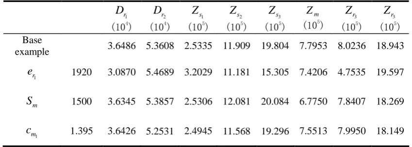
O , Or2 30. And the fixed cost for all the players are 1000. By applying the above solution procedure in section 5.2, the optimal results for the suppliers, the manufacturer and the retailers are shown in Table 1(a). In order to ensure that our conclusions are not based purely on the chosen numerical values of the base example, we also conduct some sensitive analysis on some parameters, including the market related parameter, the production related parameter and the raw material related parameter.
Through the three-level nested Nash game model and the numerical example, some meaningful managerial implications can be drawn:
(1) The increase of market parameter
1 r
e
will reduce the retailer 1’s profit, but benefit the other retailer. When1 r
e
increases, the change of the retailer 1’s demand is more sensitive to the change of his retail price compared with the base example. The retailer 1’s profit can be less reduced by lowering down his retail price. But his market demand cannot be increased, which makes the manufacturer seek for higher profit from other product to fill up the loss deduced by this product / retail market. It is good news to the other product / retailer, because the manufacturer will lower down his wholesale price to stimulate this market demand.
(2) When the manufacturer’s setup cost
S
m increases, the manufacturer’s profit decreases more significantly than the retailers’, while some suppliers’ profits increase. The increase ofS
m makes the manufacturer produce more product with higher profit margin (product 2) and reduce the production of lower profitable product (product 1). The usage of raw materials increases as the change of the manufacturer’s production strategy. At the same time, some suppliers bump up their prices, thus bringing higher profits to them.(3) The impact of the increase of supplier 1’s raw material cost
1 s
c
on his own profit may not as significant as that on the other suppliers’. The increase of1 s
c
makes the supplier 1 raise his raw material price and result in an increase cost in final products, as well as the decrease in market demands. Hence, the other suppliers will reduce their prices to keep the market and optimize their individual profits. Supplier 1 has the much lower profit margin than other suppliers, so he will not reduce his profit margin. Hence, the supplier 1’s profit decreases least.(4) When the market parameter
1 r
e
, the manufacturer’s setup costS
m, or the supplier’s raw material cost1 s
c
increase, the manufacturer’s setup time interval will be lengthened. A higher1 r
e
or1 s
decrease, as well as a lower inventory consumption rate. The increase of
S
m makes the manufacturer’s cost per production hike up. Hence, the manufacturer has to conduct his production less frequently.VI. CONCLUSION
In this paper, we have considered coordination of pricing and replenishment cycle in a multi-level supply chain composed of multiple suppliers, one single manufacturer and multiple retailers. Sensitive analysis has been conducted on market parameter, production parameter and raw material parameter. The results of the numerical example also show that: (a) when one retailer’s market becomes more sensitive to their price, his profit will be decreased, while the other retailer’s profit will increase; (b) the increase of the manufacturer’s production setup cost will bring losses to himself and the retailers, but may increase the profits of some suppliers; (c) the increase of raw material cost causes losses to all the supply chain members. Surprisingly, the profit of this raw material’s supplier may not decrease as significant as the other suppliers’; (d) the setup time interval for the manufacture will be lengthened as the increase of the retailer’s price sensitivity, the manufacturer’s setup cost or the supplier’s raw material cost.
However, this paper has the following limitations, which can be extended in the further research. Although this paper considers multiple products and multiple retailers, the competition among them is not covered. Under this competition, the demand of one product / retailer is not only the function of his own price, but also the other products’ / retailers’ prices. Secondly, the suppliers are assumed to be selected and single sourcing strategy is adopted. In fact, either supplier selection or multiple sourcing is an inevitable part of supply chain management. Also, we assume that the production rate is greater than or equal to the demand rate to avoid shortage cost. Without this assumption, the extra cost should be incorporated into the future work.
REFERENCES
[1] Boyaci, T., G. Gallego, “Coordinating pricing and inventory replenishment policies for one wholesaler and one or more geographically dispersed retailers,” International Journal of Production Economics, 77(2), 95-111, 2002.
[2] Chan, LMA, ZJM Shen, D Simchi-Levi, JL Swann, “Coordination of pricing and inventory decisions: A survey and classification,”
International Series in Operations Research and Management, Chapter 14, 2004.
[3] Esmaeili, M., Mir-Bahador Aryanezhad, P. Zeephongsekul, “A game theory approach in seller-buyer supply chain,” European Journal of Operations Research, 191(2), 442-448. 2008.
[4] Jaber, M. Y., S. K. Goyal, “Coordinating a three-level supply chain with multiple suppliers, a vendor and multiple buyer,” International Journal of Production Economics, 11(6), 95-103, 2008.
[5] Lambert, D. M, J.R. Dtock, L. M. Ellram, Fundamentals of logistics management, Boston: McGraw Hill, 1998.
[6] Liu, Baoding, “Stackelberg-Nash Equilibrium for multilevel programming with multiple followers using genetic algorithms,”
Computer Math. Application, 36(7), 79-89, 1998.
[7] Lu, L., “A one-vendor multi-buyer integrated inventory model,”
European Journal of Operational Research, 81(2), 312-323, 1995 [8] Moutaz Khouja, “Optimizing inventory decisions in a multi-stage
multi-customer supply chain,” Transportation Research Part E, 39, 193-208, 2003.
[9] Porter M., 1985, Competitive advantage: creating and sustaining superior performance, New York: The Free Press.1985
[10] Prafulla Joglekar, Madjid Tavana, Jack Rappaport, “A comprehensive set of Models of intra and inter-organizational coordination for marketing and inventory decisions in a supply chain,” International Journal of Integrated Supply Management, 2006.
[11] Simchi-Levi, D., Kaminsky, P., Simchi-Levi, E., Designing and managing the supply chain, Irwin McGraw-Hill, New York, 2000 [12] Weng, Z.K, “Channel coordination and quantity discounts,”
Management Science, 41(9), 1509-1522, 1995.
[13] Weng, Z.K, R.T. Wong, “General models for the supplier’s all-unit quantity discount policy,” Naval Research Logistics, 40(7), 971-991, 1993.
[14] Woo Y. Y., Shu-Lu Hsu, Soushan Wu, “An integrated inventory model for a single vendor and multiple buyers with ordering cost reduction,”
International Journal of Production Economics, 73, 203-215, 2001. [15] Yu Yugang, Liang Liang, George Q. Huang, “Leader-follower game in
(a) Product demand and profits for suppliers, manufacturer and retailers
1 r
D
(104
)
2 r
D
(104
)
1 s
Z
(105
)
2 s
Z
(105
)
3 s
Z
(105
)
m
Z
(105
)
3 r
Z
(105
)
3 r
Z
(105
) Base
example 3.6486 5.3608 2.5335 11.909 19.804 7.7953 8.0236 18.943
1 r
e
1920 3.0870 5.4689 3.2029 11.181 15.305 7.4206 4.7535 19.597m
S
1500 3.6345 5.3857 2.5306 12.081 20.084 6.7750 7.8407 18.2691 m
c
1.395 3.6426 5.2531 2.4945 11.568 19.296 7.5513 7.9950 18.149(b) Pricing and replenishment decisions for suppliers, manufacturer and retailers
1 s
p
2 s
p
3 s
p
pm1p
m2p
r3p
r3K
s1K
s2K
s3k
r1k
r2T
1.77 6.15 15.15 79.37 101.96 102.20 140.28 1 1 2 6 11 0.2691
1.99 5.99 13.58 71.98 100.42 88.09 139.51 1 1 2 6 11 0.2695
1.76 6.20 15.27 79.55 101.61 102.28 140.10 1 1 1 7 14 0.3252
[image:6.595.84.509.91.243.2]2.23 6.09 15.01 79.44 103.50 102.23 141.05 1 1 2 6 11 0.2707