Munich Personal RePEc Archive
Economic Growth, Financial
Development and Income Inequality in
BRICS Countries: Evidence from Panel
Granger Causality Tests
Younsi, Moheddine and Bechtini, Marwa
Faculty of Economics and Management, University of Sfax, Tunisia
13 March 2018
Online at
https://mpra.ub.uni-muenchen.de/85251/
1
Economic Growth, Financial Development and Income Inequality in
BRICS Countries: Evidence from Panel Granger Causality Tests
By
Moheddine YOUNSI
a†& Marwa BECHTINI
bAbstract
The purpose of this paper is to examine the causal relationship between economic growth, financial development and income inequality for the BRICS countries, namely; Brazil, Russia, India, China, and South Africa, using annual panel data covering the period 1995-2015. We construct a composite financial sector development index for these countries by applying the principal component method on the main four proxies of financial development, that is, domestic credit to private sector to GDP ratio, domestic credit given by banks sector to GDP ratio, M2/GDP, and stock market capitalization to GDP ratio. Results of Pedroni panel cointegration and Kao residual panel cointegration tests confirm the valid long-run cointegration relationship between the considered variables. Fixed effects estimation results show that GDP per capita growth has a positive and significant effect on income inequality, while the coefficient of its squared term has negative and significant effect on income inequality. Similarly, financial development index appears to have a positive and statistically significant effect on income inequality, while its squared term has negative and statistically significant effect on income inequality. Our empirical findings support the financial Kuznets hypothesis of an inverted U-shaped relationship between economic growth, financial sector development and inequality in the BRICS countries over the study period. Our results are robust by employing POLS and GMM estimators. Results of Granger causality test shown that there is a unidirectional causality running from financial development index to income inequality, but a bidirectional causality between inflation and income inequality is found. However, there is no causal relationship between income inequality and economic growth. These findings are expected to help policymakers to reduce inequality in these countries through the improvement of taxation policies financial system.
Keywords: Economic growth, financial development, income inequality, financial Kuznets hypothesis, BRICS countries.
JEL-Classification: D63, G20, O11
a†
Unit of Research in Development Economics, Faculty of Economics and Management, University of Sfax, Tunisia.
E-mail address: [email protected]
b
Unit of Research in Competitiveness, Commercial Decision and Internationalization, Faculty of Economics and Management, University of Sfax, Tunisia.
2
1. Introduction
It is widely argued that strong financial sector development plays a vital role in promoting economic growth and reducing income inequality and poverty. However, several exiting studies provide evidence on the important role play by the finance and sound financial system as they contributes to economic development through increasing total productivity, promoting economic competitiveness and encouraging market-driven dynamic (McKinnon, 1973; Shaw, 1973; Levine, 1997; Levine et al., 2000). Likewise, other empirical studies suggest that well-developed financial sector contributes to alleviate largely income inequality and stimulate economic growth (;Beck et al., 2007; Agnello and Sousa, 2012; Jalil and Feridun, 2011; Hoi and Hoi, 2013; Nikoloski, 2013; Shahbaz et al., 2015; Satti et al., 2015; Zhang and Cheng, 2015). It is emphasized that a well-developed financial sector may offer inexpensive credit and easing access to financial services to the various people that helps to improve entrepreneurial activities which hence create job opportunities and enhance welfare of the society. Therefore, improving access to credit at lower cost can provide decisive support to financially poor families by allowing them to invest in health and education, thereby promoting the human capital formation in the economy, which will certainly contribute to the distribution of income and poverty reduction.
It is a well-known fact that financial sector development has obviously contributed to the striking economic growth of many emergent countries like the case of the BRICS countries (Brazil, Russia, India, China, and South Africa), which have undergone profound economic and social changes over the last few decades. In addition to their rapid economic growth which reaches, for example, in China about 6.9% and in India about 7.5% in 2015, reducing inequality in these countries is one of the most important issues to maintain their economic, political and social stability. It is widely argued that economic growth is the most powerful driver for reducing inequality (Bruno et al., 1998). However, the positive effects of growth are reduced by increasing inequality in some countries. It is emphasized in the literature that an effective financial system is important for enhancing growth and economic development. Many empirical studies have shown that scarce financial markets can be a source of income inequality and that financial sector imperfections creates income inequality, by assisting entrepreneurs and hurting lenders through its effect of decreasing the rental rate of capital (Westley, 2001; Mookherjee and Ray, 2003; Hye and Islam, 2013; Daisaka et al., 2014, Satti et al., 2015). It is not surprisingly that the phenomenon of income inequality has been upsurge worldwide and it affects almost all the developed, emerging and developing countries, whereas social welfare of the people depends negatively on the level of inequality of a country. Overall, extensive income inequality may generate serious adverse effects on the economy like slowing down economic growth, increasing unemployment and social tensions. Therefore, to stimulate economic growth and alleviate income inequality a sound financial sector development is required.
Although there is a growing body of studies on the relation between financial development and income inequality, the relationship between economic growth, financial sector development and inequality in the context of the BRICS countries is yet not well explored. Hence, the main objective of this paper is to empirically examine the causal relationship among economic growth, financial development and income inequality and tested the existence of Kuznets curve hypothesis (Kuznets, 1955), which illustrates an inverted U-shaped linkage between economic growth, financial development and inequality, in BRICS countries. To this end, we use annual panel data for BRICS countries covering 1995-2015. This study contributes to the literature on the relationship between financial development and inequality by using different techniques, time period and combination of explanatory variables, which are relatively different as compared to the previous empirical studies. We expect that the outcomes of this paper may help the policy makers to alleviate inequality through the development of financial system.
3
2. Literature Review
The dynamic relationship between financial development and income inequality has received considerable attention since the last few decades. However, many papers have been appeared the last few years covering various geographic locations, using different econometric tools and including a range of control variables. Numerous empirical studies have focused on a specific-country while others have relied on a group of countries within a panel data framework, using different methodologies and time period, and have found conflicting results.
At a cross-country level, Li et al. (1998) examined the dynamic link between financial development and income inequality for a group of 49 developed and developing countries during the period 1947-1994 by using various estimation techniques. Their empirical results show a strong relationship between financial development and income inequality. Clarke et al. (2006) examined the link between financial development and income inequality for a sample of 83 countries over the period 1960-1995 using a dynamic panel model. Their evidence strongly supports the negative linear hypothesis which assets that financial development plays a vital role to improve growth and reduce income inequality. Using a similar model and panel dataset on income inequality for 72 countries from 1960 to 2005,
Beck et al. (2007) find that developed financial sector helps to increase the incomes of the poorest
quintile. Their interesting findings is that, at the long-run, around 40% of the influence of financial development on income growth of the poorest quintile is as a result of the declines in income inequality, whereas 60% is the results of the influence of financial development on economic growth as a whole. Meanwhile, Rehman et al. (2008) used a panel data for 51 unbalanced countries over the period 1975-2002 to analyze the factors driving income inequality. For testing the Kuznets hypothesis, the authors divided panel data into four sub-panels of income group counties according to their stages of economic growth: low income, low-middle income, upper-middle income and high income. The empirical results confirm the presence of an inverted U-shaped hypothesis for income per capita growth in all income groups, but they find no evidence supporting the Kuznets hypothesis of an inverted U-shaped association between financial development and income inequality.
Using a panel dataset covering 22 African countries from 1990 to 2004, Batuo et al. (2010) examined the influence of financial development on income inequality by testing various theoretical hypotheses. However, this study fails to confirm the Greenwood-Jovanovic (1990) hypothesis of an inverted U-shaped relationship between financial development and income inequality in these countries. Kappel (2010) investigated the effects of financial development on income inequality and poverty for a panel of 78 developing and developed countries for the period 1960-2006, using Two-Stage Least Squares (2SLS) regression analysis. The empirical results indicate that financial development remains to have a negative and significant effect on inequality for medium- and high income countries, but there is no significant effect on low-income countries. This study thus highlights that inequality and poverty are not only reduced through improved loan market but also as well as through developed stock market. In a similar study, Kim and Lin (2011) used data for 65 countries during the period 1960-2005. Their results based on panel threshold regressions reveal that the benefits of financial development on income distribution only occur if the state has reached a threshold level and below this critical threshold the financial development tends to worsen income distribution.
4 over the period 1962-2006 by employing multivariate dynamic panel regression models. The empirical findings lend support for the feedback hypothesis of Greenwood-Jovanovic of an inverted U-shaped relationship between financial development and income inequality. Law et al. (2014) used a panel threshold regression approach for testing the effect of financial development on income inequality at different institutional quality levels for 81 countries during the period 1985-2010. They observe that financial development serves to alleviate income inequality only after a certain threshold scale of institutional quality has been achieved and suggest that until then the threshold effect of financial development on income inequality is nonexistent. Using time series data regressions for 17 countries, Bahmani and Zhang (2015) examined the short-run dynamics and long-run equilibrium relationship among financial development and income distribution and find mixed results. However, the short-run impacts of financial market development on income distribution are found to be equalizing in 10 counties, while, the equalizing impacts persisted into the long-run only in three out of the 10 countries, that is, Denmark, Kenya and Turkey.
Next to cross-country studies, there exists also various country-specific investigation. However, Burgess and Rohini (2005) investigated the effect of rural bank openings on poverty in Indian states with lower initial financial development between 1961 and 2000. Their results suggest that opening of bank branches in country side/rural areas facilitated improving income distribution. They also found that rural bank sectors expansion and savings mobilization serves to boost total per capita output. Using annual time series data from 1951 to 2004 and the error correction model, Ang (2010) examined the impact of financial development on income inequality in India. His study does not find any evidence about the Kuznets hypothesis of an inverted U-shaped relationship between financial development and income inequality in India. Consistently, Giri and Sehrawat (2015) applied the ARDL bounds testing approach to cointegration and the error correction model in order to examine the long-run and short-run relationship between financial development and income inequality in India. It covers annual data from 1982 to 2012. The cointegration test results indicate a long-run cointegration relationship between financial development and income inequality. The ARDL test results provide evidence that financial development worsens income inequality in both short-run and long-run rather widen the gap between poor and rich.
5 development and income inequality in Malaysia during the period 1970-2007. The results of empirical tests from ARDL approach show that financial development is found to be statistically insignificant in reducing income inequality in Malaysia. Odhiambo (2010) examined the dynamic relationship between financial development, investment and economic growth in South Africa by applying the ARDL bounds testing approach to cointegration for the period 1969 2006 and find that economic growth has a substantially supportive influence on the financial sector development when private credit to GDP ratio, liquid liabilities to GDP ratio and M2/GDP are used as measures for financial development. In the case of Pakistan, Shahbaz and Islam (2011) examined the dynamic relationship between financial development and income inequality in Pakistan for the period from 1971 to 2005 with the ARDL bounds testing approach to cointegration and error correction model (ECM). The empirical evidence shows that financial development significantly contributes to decrease income inequality whilst economic growth exacerbates income distribution for the period under study thereby rejecting the existence of financial Kuznets curve hypothesis.
By employing a sample of provincial panel data from 2002 to 2008, Hoi and Hoi (2013) explored the link between financial development and income inequality in Vietnam. Their empirical evidence suggests that financial development when it interacts with educational attainment channel has shared-influences on reducing income inequality in Vietnam. However, the study fails to confirm the inverted U-shaped relationship between the financial development and income inequality. In a similarly related cross-provincial study, Hoi and Hoi (2016) investigated the dynamic relationship between financial development and income inequality in Vietnam from 2002 to 2012 by using the GMM estimator. They find that financial market expansion increases in inequality. In line with Hoi and Hoi (2013), their findings are inconsistent with the Greenwood-Jovanovic hypothesis of an inverted U-shaped relationship between financial development and income inequality. In the case of Iran, Shahbaz et al. (2015) applied the ARDL bounds testing approach and vector error correction model (VECM) Granger causality to examine the dynamic causal relationship between financial development and income inequality for the period 1965-2011.The empirical results provide strong evidence of an inverted U-shaped relationship between financial development and income inequality, while there is supporting evidence for U-shaped relationship between globalization and income inequality. In the same vein, Shahbaz et al. (2017) look into the long-run relationship between financial development and income inequality in Kazakhstan for the period 1991-2011. Their empirical results based on the ARDL bounds tests indicate the existence of a long run connection between financial development and income inequality. Therefore, the empirical results suggest the decreasing effect of financial development on income inequality, while economic growth exacerbates income inequality, whereas both inflation and trade openness increase income distributionfor the period under study.
3. Methodology
3.1. Data
6
3.2. Model Specification
To examine the relationship between economic growth, financial development and income inequality, we consider the baseline model as follows:
(1)
where i = 1,…, N represents countries observed over the periods t = 1,…, T, Gini is the Gini coefficient which measures income inequality, GDP is per capita income growth, GDP2 is its squared term, INF is inflation rate, FDI is the composite financial sector development index, FDI2 is its squared term for analyzing the existence of financial Kuznets hypothesis for BRICS countries, and εis the error term.
In order to analyze the stationary properties of the relevant variables, we begin our framework by performing the panel unit root tests proposed by Levin, Lin and Chu (LLC) (2002), and Im, Pesaran
and Shin (IPS) (2003). The starting point of LLC (2002) is to assume that the stochastic process is
generated by the first order autoregressive process as:
(2)
where is the corresponding panel data series in difference term, α = -1, is the lag order for that may fall and rise for cross section and is the exogenous variable in the model. The LLC
(2002) unit root test consider that the different autoregressive parameters as homogeneous across all
individuals i.e. for all i. The null hypothesis under the LLC (2002) is that each series have a unit root, for all i against the alternative hypothesis that some of the individual series has a unit root, for all i. The asymptotic distribution of these statistics follows a standard normal distribution. The individual unit root procedure is allowed in IPS (2003) panel unit root test. Hence, the IPS unit root test combines the individual unit root test to derive a panel specific result.
After confirming that all series in our panel are integrated with order one, the next step is to test for the presence of cointegration among them. To this end, we use Pedroni (1999) panel cointegration technique to examine the long-run relationship between the variables. This technique is preferred over other cointegration methods of its class because it is usefully effective for controlling the country’s size bias and solving the heterogeneity issue through parameters that may differ among individuals. However, to test for cointegration in a heterogeneous panel data, Pedroni (1999) consider the following cointegrating regression:
(3)
where αi is the country specific fixed effects and δit represents country specific time trends, which
captures any country specific omitted variables. The slope coefficients β1i, β2i, β3i and β4i can differ
from one individual to another allowing the cointegrating vectors to be heterogeneous a cross countries. The estimated residuals are as the following form:
(4)
Under the null hypothesis of no cointegration, that is, . There are two alternative hypotheses. First, the homogenous alternative (within dimension or panel statistics) to be tested as
. Second, the heterogeneous alternative (between dimension or group statistics) to be tested is
.
7
3.3. Construction of a Composite Financial Development Index
To analyze the importance of financial reforms on the performance of any economy, researchers applied two different methods. The first group of researchers used different proxies of financial sector development to analyze the utilization of different financial reforms features and characteristics on the performance of the economy (e.g. Ahmed, 2007; Bittencourt, 2010; Hye, 2011). The second group of researchers deals with constructing a synthetic financial sector development index by applying the principal component analysis (PCA) method on the major measures of financial development (e.g. Batuo et al. , 2010; Hye and Islam, 2013). Following, Batuo et al. (2010) and Hye and Islam (2013), we construct a composite financial sector development index for the Brazil, Russia, India, China, and South Africa economies by applying the principal component analysis (PCA) method on the our main measures of financial development, namely; domestic credit to private sector to GDP ratio, domestic credit given by banks sector to GDP ratio, broad money supply (M2) to GDP ratio and stock market capitalization to GDP ratio. The PCA is a multivariate statistical technique which usually used for analyzing the inter-correlation linking several quantitative variables. In terms of methodology, for each dataset with p quantitative variables, we can evaluate at most p principal components (PC), each being a linear combination of the original variables, where the coefficients are equal to the eigenvectors of the correlation covariance matrix. The PC is then arranged by descending order of the eigenvalues which are equal to the variance of the components.
The results of construction of the composite of financial sector development index for Brazil, Russia, India, China, and South Africa through PCA method are reported in Appendix A1. The PC analysis for Brazil indicate that the first PC explains about 70.21%, the second PC explains 27.18%, the third PC explains 1.96% and the fourth PC explains 0.65% of the standardized variance. This implies that we select the first PC to compute the financial development index. The first PC is a linear combination of the four measures of financial development with weights provided by the first eigenvector. After rescaling, the individual contributions of each series DCB, DCP, M2 and SMC to the standardized variance of the first PC are around 59.99%, 58.81%, 36.97%, and 41.15%, respectively. We use further these weights to construct the composite financial sector development index for the economy of Brazil. The same interpretation of the results is found to be true regarding the economy of Russia, India, China and South Africa.
4. Empirical Results
4.1. Descriptive Statistics
8
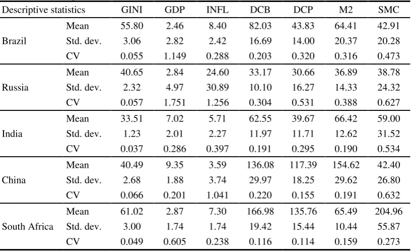
Table 1. Descriptive statistics
Descriptive statistics GINI GDP INFL DCB DCP M2 SMC
Mean 55.80 2.46 8.40 82.03 43.83 64.41 42.91 Brazil Std. dev. 3.06 2.82 2.42 16.69 14.00 20.37 20.28 CV 0.055 1.149 0.288 0.203 0.320 0.316 0.473
Mean 40.65 2.84 24.60 33.17 30.66 36.89 38.78 Russia Std. dev. 2.32 4.97 30.89 10.10 16.27 14.33 24.32 CV 0.057 1.751 1.256 0.304 0.531 0.388 0.627
Mean 33.51 7.02 5.71 62.55 39.67 66.42 59.00 India Std. dev. 1.23 2.01 2.27 11.97 11.71 12.62 31.52 CV 0.037 0.286 0.397 0.191 0.295 0.190 0.534
Mean 40.49 9.35 3.59 136.08 117.39 154.62 42.40 China Std. dev. 2.68 1.88 3.74 29.97 18.25 29.62 26.80 CV 0.066 0.201 1.041 0.220 0.155 0.191 0.632
Mean 61.02 2.87 7.30 166.98 135.76 65.49 204.96 South Africa Std. dev. 3.00 1.74 1.74 19.42 15.44 10.44 55.87
CV 0.049 0.605 0.238 0.116 0.114 0.159 0.273
Notes: Std. dev. indicates standard deviation, CV: indicates coefficient of variation.
Source: Authors' estimations based on WDI database.
4.2. Results of Panel Unit Root and Cointegration Tests
In this study, we begin our data analysis by checking the stationary properties of the relevant variables, for this purpose, we use Levin, Lin and Chu (LLC) (2002), and Im, Pesaran and Shin (IPS) (2003) panel unit root tests. Table 2 reports the results of panel unit root tests. These tests are first applied on the level of variables, then on their first difference. The null hypothesis of non-stationarity based on both the LLC and IPS tests is rejected against the alternative hypothesis at the 1% level of significance, indicating that all series in our panel sets are stationary and integrated at their first difference, I(1), with intercept, and with intercept and trend. These results provide strong evidence that the series of variables may exhibit no unit root problem and we can then use them to analyze the long-run relationship.
Table 2. Panel unit root tests results
Levin, Lin & Chu test Im, Pesaran and Shin test
Variables Level First difference Level First difference
I I&T I I&T I I&T I I&T
GINI -0.625 -1.637 -7.420*** -6.635*** -1.257 -1.527 -8.669*** -7.553*** GDP 0.430 0.846 -6.374*** -3.768*** 0.077 4.173 -5.317*** -3.970*** INFL 1.413 3.072 -3.930*** -2.698*** -2.134 -2.261 -7.158*** -5.858*** FDI 2.284 -0.269 -5.523*** -4.914*** 4.303 1.224 -4.788*** -4.104***
Notes: *, ** and *** denote significance at the 10%, 5% and 1% levels, respectively, I indicates intercept,
I &T indicate intercept and trend.
Source: Authors' estimations.
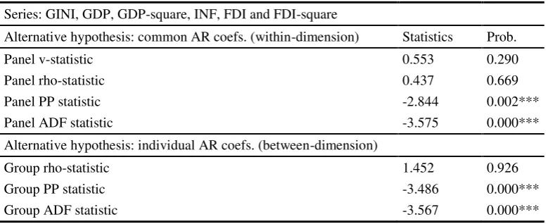
[image:9.595.68.515.540.650.2]9 Results show that the augmented Dickey-Fuller (ADF) and Phillips-Perron (PP) tests statistics based on both within dimension and group based approach statistics reject the null hypothesis of no cointegration. Thus, it is concluded that all variables are cointegrated and exhibited a valid long-run relationship.
Table 3. Pedroni panel cointegration tests
Series: GINI, GDP, GDP-square, INF, FDI and FDI-square
Alternative hypothesis: common AR coefs. (within-dimension) Statistics Prob.
Panel v-statistic 0.553 0.290
Panel rho-statistic 0.437 0.669
Panel PP statistic -2.844 0.002***
Panel ADF statistic -3.575 0.000***
Alternative hypothesis: individual AR coefs. (between-dimension)
Group rho-statistic 1.452 0.926
Group PP statistic -3.486 0.000***
Group ADF statistic -3.567 0.000***
Notes: *** indicates the rejection of the null hypothesis at the 1% significance level.
The null hypothesis of Pedroni’s test is that the variables are not cointegrated.
Source: Authors' estimations.
Kao residual cointegration test is reported in Table 4. Results indicate the rejection of null hypothesis of no cointegration at the 5% level of significance, which implies there exists a long-run cointegration relationship between the considered variables.
Table 4. Kao residual cointegration test
Model specification: No deterministic trend
ADF t-statistics -1.712 (0.043)**
Notes: ** indicates the rejection of the null hypothesis at the 5% significance level.
Source: Authors' estimations.
4.3. Results and Robustness Checks
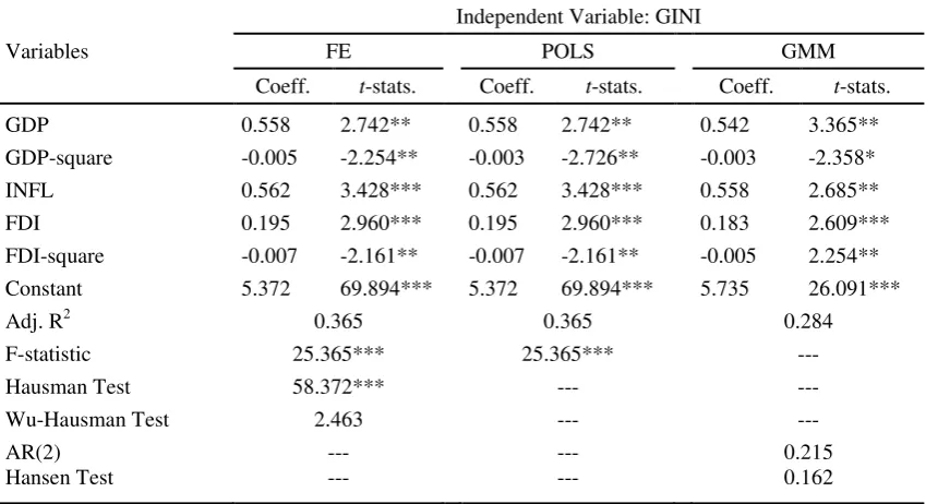
[image:10.595.72.401.432.465.2]10 Based on the above diagnostic tests, which confirm that fixed effects method is preferred for our analysis, we estimate our baseline model by using a panel data regression with fixed effects. Results of income inequality equation with fixed effects estimation are presented in Table 5 in Column (1). Our empirical evidence shows that the financial development index has positive and statistically significant effect on income inequality in BRICS countries, while the coefficient of its square-term has a negative and statistically significant effect on income inequality at 1% level. The magnitude of 0.195 implies that a 1% increase in financial development decreases income inequality by around 0.195%. This result suggests that a well-functioning financial sector system is essential for promoting economic and reducing income inequality by increasing the availability of financial services to the poor for financing their capital investments.
Similarly, GDP per capita growth appears to have a positive and statistically significant impact on income inequality, while the coefficient of its square-term has negative and significant impact on income inequality at 5% level. The magnitude of 0.558 indicates that a 1% increase in per capita GDP growth increases income inequality by 0.558%, suggesting that when GDP per capita growth continues to increase, income inequality starts to decrease. The estimates also show as well that inflation has a positive and significant impact on income inequality at the 1% significance level. This result implies that when macroeconomic stability improved by decreasing inflation, financial development became more effective in reducing inequality. These findings support the Kuznets hypothesis of an inverted U-shaped relationship between economic growth, financial development and income inequality in BRICS countries.
In order to assess the robustness of our results, we use the pooled ordinary least square (POLS) and the GMM estimators. The GMM is the estimation technique most usually applied in models with panel data and in the multiple-way linkages between the explanatory variables. This approach utilizes a set of instrumental variables (IV) to solve the endogeneity problem. According to Arrellano and Bond (1991), and Blundell and Bond (1998), two specific diagnostic tests are used to examine the soundness of the instruments. First, Hansen test was used to test the over-identifying restrictions in order to provide some evidence of the instruments' validity. The null hypothesis of the Hansen test is that all instruments are uncorrelated with the error term. The second diagnostic test is the second-order autocorrelation AR (2) test, which checks for serial correlations of the error terms (Arellano and Bond, 1991).
11
Table 5. The estimation results of FE, POLS and GMM
Variables
Independent Variable: GINI
FE POLS GMM
Coeff. t-stats. Coeff. t-stats. Coeff. t-stats.
GDP 0.558 2.742** 0.558 2.742** 0.542 3.365**
GDP-square -0.005 -2.254** -0.003 -2.726** -0.003 -2.358* INFL 0.562 3.428*** 0.562 3.428*** 0.558 2.685**
FDI 0.195 2.960*** 0.195 2.960*** 0.183 2.609***
FDI-square -0.007 -2.161** -0.007 -2.161** -0.005 2.254** Constant 5.372 69.894*** 5.372 69.894*** 5.735 26.091***
Adj. R2 0.365 0.365 0.284
F-statistic 25.365*** 25.365*** ---
Hausman Test 58.372*** --- ---
Wu-Hausman Test 2.463 --- ---
AR(2) --- --- 0.215
Hansen Test --- --- 0.162
Notes: Robustness analysis is checked using POLS and GMM estimators. Hansen test refers to the over-identification test for
the restrictions in GMM estimation.
*, **, *** indicate significance at the 1%, 5%, and 10% levels, respectively.
Source: Authors' estimations.
4.3. Granger Causality Analysis
Finally, to examine the causality direction between economic growth, financial development and income inequality, we use panel Granger causality test. Granger Causality is a statistical hypothesis test which verifies whether one time series is skilled of forecasting another (Granger, 1969). Granger causality is a powerful tool for analyzing the causal effect and functional link from various panel data. We determine the causality analysis of the income inequality equation on lag one. According to Jones (1989), ad-hoc selection technique for lag length in Granger causality test is most preferred to other statistical technique to determine the optimal lag length.
[image:12.595.66.419.595.705.2]Table 6 reports the results of Granger causality test. Results show that there is a unidirectional causality running from financial development index to income inequality, but a bidirectional causality running from inflation to income inequality and from income inequality to inflation is found. This implies that inflation and income inequality both are significantly affecting each other. However, there is no causal relationship between income inequality and economic growth.
Table 6. Panel Granger causality results
Variables F-statistics Prob.
GDP does not Granger cause GINI 1.554 0.113
GINI does not Granger cause GDP 1.941 0.166
INFL does not Granger cause GINI 4.637 0.033
GINI does not Granger cause INFL 3.020 0.085
FDI does not Granger cause GINI 4.768 0.031
GINI does not Granger cause FDI 2.459 0.120
Notes:The lag length of all variables is 1.
12
5. Conclusions and Policy Implications
This paper seeks to strengthen the existing literature by examining the link between economic growth, financial development and income inequality for 5 emerging countries, namely; Brazil, Russia, India, China, and South Africa by using annual panel data covering the period 1995-2015. We construct a composite financial sector development index for our simple countries by applying the principal component method on the main four proxies of financial development, that is, domestic credit to private sector to GDP ratio, domestic credit given by banks sector to GDP ratio, M2/GDP, and stock market capitalization to GDP ratio. The analysis of the three-way linkages between economic growth, financial development and income inequality in BRICS countries yields a number of significant and interesting results. However, Pedroni panel cointegration and Kao residual panel cointegration tests results confirm the valid long-run cointegrating relationship between our considered variables. The results of fixed effects model indicate that financial development index has a positive and statistically significant impact on income inequality, while its squared-term has a negative and statistically significant influence on income inequality. Likewise, GDP per capita growth has a positive and significant effect on income inequality, while the coefficient of its squared-term appears to have a negative and significant influence on income inequality in these countries during the sample period. Inflation is found to be positive and significant. Our findings confirm the financial Kuznets hypothesis of an inverted U-shaped relationship between economic growth, financial development and income inequality in the BRICS countries during the period 1995-2015. These results are robust by employing POLS and GMM estimators.
The salient policy implication of our findings suggests that to reduce income inequality in the sample countries. The policy makers forcefully need to devise fiscal policy and thereby progressive taxes in the true sense. It should be noted that public spending especially on education is more effective than taxation policies in addressing inequality. However, the development of education reduces inequality of labor income by increasing the supply of more skilled workers and public education can make education less dependent on personal and social conditions and serves to balance the human capital accumulation across the poor and the rich thereby reducing income inequality. The governments should be forcefully promoting inclusive development covering policies of rural development, including financial services and income tax policies. Likewise, the government needs to subsidized essential foodstuffs particularly for the poor to reduce burden on the poor people. Progressive redistribution of asset ownership plan plays also a key role in reducing income inequality. Finally, to tackle inequality in BRICS, the government’s efforts are required to enhance their quality of institutions, targeting inflation level and reinforce further their financial systems.
References
Agnello, L., Sousa, R. M. 2012. How do banking crises impact on income inequality? Applied Economics Letters 19(15): 1425-1429.
Ahmed, A. D. 2007. Potential impact of financial reforms on savings in Botswana: an empirical analysis using a VECM approach. The Journal of Developing Areas 41(1): 203-220.
Ang, J. B. 2010. Finance and inequality: the case of India. Southern Economic Journal 76(3): 738-761.
Arellano, M., Bond, S. 1991. Some Tests of Specification for Panel Data: Monte Carlo Evidence and an Application to Employment Equations. The Review of Economic Studies 58(2): 277-297.
13 Batuo, M., Mlambo, K., Guidi, F. 2010. Financial development and income inequality: Evidence from African Countries. MPRA Paper No. 25658. http://mpra.ub.uni-muenchen.de/25658
Beck, T., Demirguç-Kunt, A., Levine, R. 2007. Finance, inequality and the poor. Journal of Economic Growth 12(1): 27-49.
Bittencourt, M. 2010. Financial development and inequality: Brazil 1985-99. Economic Change and Restructuring 43(2): 113-130.
Blundell, R., Bond, S. 1998. Initial conditions and moment restrictions in dynamic panel data models. Journal of Econometrics 87(1): 115-143.
Burgess R., Rohini, P. 2005. Do Rural Banks Matter? Evidence from the Indian Social Banking Experiment. American Economic Review 95(3): 780-795.
Clarke, G. R., Xu, L. C., Zou, H-F. 2006. Finance and Income Inequality: What Do the Data Tell Us? Southern Economic Journal 72(3): 578-596.
Clarke, G., Xu. L. C., Zou, H-F. 2013. Finance and Income Inequality: Test of Alternative Theories. Annals of Economics and Finance 14-2(A): 493-510.
Daisaka, H., Furusawa, T., Yanagawa, N. 2014. Globalization, Financial Development and Income Inequality. Pacific Economic Review 19(5): 612-633.
Giri, A. K., Sehrawat, M. 2015. Financial development and income inequality in India: An application of ARDL approach. International Journal of Social Economics 42(1): 64-81.
Granger, C. W. J. 1969. Investigating Causal Relations by Econometric Models and Cross-spectral Methods. Econometrica 37(3): 424-438.
Greene, W. H. 2000. Econometric Analysis. Upper Saddle River, N.J.: Prentice Hall.
Greenwood, J., Javanovic, B. 1990. Financial Development, Growth and Distribution of Income. Journal of Political Economy 98(5): 1076-1107.
Gujarati, D. 2003. Basic econometrics. Singapore: McGraw-Hill Companies, Inc.
Hausman, J. A. 1978. Specification tests in econometrics. Econometrica 46(6): 1251-1272.
Hoi, L. Q., Hoi, C. M. 2013. Financial Sector Development and Income Inequality in Vietnam: Evidence at the Provincial Level. Journal of Southeast Asian Economies 30(3): 263-277.
Hoi, L. Q., Hoi, C. H. 2016. Credit Market Depth and Income Inequality in Vietnam: A Panel-Data Analysis. Journal of Economics and Development 18(2): 5-18.
Hye, Q. M. A. 2011. Financial development index and economic growth: empirical evidence from India. The Journal of Risk Finance 12(2): 98-111.
Hye, Q. M. A., Islam, F. 2013. Does financial development hamper economic growth: empirical evidence from Bangladesh. Journal of Business Economics and Management 14(3): 558-582.
14 Jalil, A., Feridun, M. 2011. Long-run relationship between income inequality and financial development in China. Journal of the Asia Pacific Economy 16(2): 202-214.
Kao, C. 1999. Spurious regression and residual-based tests for cointegration in panel data. Journal of Econometrics 90(1): 1-44.
Kappel, V. 2010. The effects of financial development on income inequality and poverty. Working Paper, 10/127, CER-ETH-Center of Economic Research at ETH Zurich.
Kim, D. H., Lin., S. C. 2011. Nonlinearity in the financial development and income inequality nexus. Journal of Comparative Economics 39(3): 310-325.
Kuznets, S. 1955. Economic Growth and Income Inequality. American Economic Review 45 (1): 1-28.
Law, S. H., Azman-Saini, W. N., Tan, H. B. 2014. Financial Development and Income Inequality at Different Levels of Institutional Quality. Emerging Markets Finance and Trade 50(1): 21-33.
Levine, R. 1997. Financial Development and Economic Growth: Views and Agenda. Journal of Economic Literature 35(2): 688-726.
Levine, R., Beck, T., Loayza, N. 2000. Financial intermediation and growth: Causality and causes. Journal of Monetary Economics 46(1): 31-77.
Levin, A., Lin, C. F., Chu, C. S. 2002. Unit root tests in panel data: asymptotic and finite-sample properties. Journal of Econometrics 108(1): 1-24.
Li, H., Squire, L., Zou, H. F. 1998. Explaining International and Intertemporal Variations in Income Inequality. The Economic Journal 108(446): 26-43.
Liang, Z. 2006a. Financial development and income inequality in rural China 1991-2000. Research Paper No. 2006/96. United Nation University-World Institute for Development Economics Research (UNU- WIDER), Helsinki. http://hdl.handle.net/10419/63268
Liang, Z. 2006b. Financial development and income distribution: A system GMM panel analysis with application to urban China. Journal of Economic Development 31(2): 1-21.
Ling-Zheng, Y., Xia-Hai, W. 2012. Has financial development worsened income inequality in China? Evidence from threshold regression model. Journal of Finance and Economics, CNKI-SUN: CJYJ.0.2012-03-009.
Mansur, M., Azleen, R. 2017. What is the link between financial development and income inequality? Evidence from Malaysia. MPRA Paper No. 79416. http://mpra.ub.uni-muenchen.de/79416
McKinnon, R. I. 1973. Money and capital in economic development. Brookings Institution Press.
Mookherjee, D., Ray, D. 2003. Persistent Inequality. The Review of Economic Studies 70(2): 369-393.
Nikoloski, Z. 2013. Financial sector development and inequality: is there a financial Kuznets curve? Journal of International Development 25(7): 897-911.
Odhiambo, N. M. 2010. Finance-investment-growth nexus in South Africa: an ARDL bounds testing procedure. Economic Change and Reconstructing 43(3): 205-219.
15 Rehman, H., Khan, S., Ahmed, I. 2008. Income distribution, growth and financial development: a cross countries analysis. Pakistan Economic and Social Review 46(1): 1-16.
Shahbaz, M., Islam, F. 2011. Financial development and income inequality in Pakistan: An application of ARDL approach. Journal of Economic Development 36(1): 35-58.
Shahbaz, M., Loganathan, N., Tiwari, A. K., Sherafatian-Jahromi, R. 2015. Financial Development and Income Inequality: Is There Any Financial Kuznets Curve in Iran? Social Indicators Research 124(2): 357-382.
Shahbaz, M., Bhattacharya, M., Mahalik, M. K. 2017. Finance and income inequality in Kazakhstan: Evidence since transition with policy suggestions. Applied Economics 49(52): 5337-5351.
Shaw, E. S. 1973. Financial deepening in economic development. New York: Oxford University Press.
Tan, H. B., Law, S. H. 2009. The role of financial development on income inequality in Malaysia. Journal of Economic Development 34(2): 153-168.
Tan, H. B., Law, S. H. 2012. Nonlinear dynamics of the finance-inequality nexus in developing countries. Journal of Economic Inequality 10(4): 551-563.
Westley, G. D. 2001. Can Financial Market Policies Reduce Income Inequality? Technical Paper Series, No. MSM-112. Inter-American Development Bank, Washington, D.C.
WDI. 2016. World Development Indicators. World Bank. http://data.worldbank.org/indicator
16
Appendix A1. Construction of Financial Development Index for Brazil, China, India, Russia and South Africa
Brazil Eigenvalues (Sum = 4, Average = 1) Eigenvectors (loadings) Number Value Difference Proportion
Cumulative Value
Cumulative
Proportion Variable PC 1 PC 2 PC 3 PC 4
1 2.808432 1.721389 0.7021 2.808432 0.7021 DCB 0.589964 -0.013428 -0.319431 -0.741435 2 1.087044 1.008528 0.2718 3.895476 0.9739 DCP 0.588119 0.022192 -0.459197 0.665403 3 0.078516 0.052508 0.0196 3.973992 0.9935 MS 0.369761 0.737347 0.564060 0.037854 4 0.026008 --- 0.0065 4.000000 1.0000 SMC 0.411503 -0.675016 0.607402 0.077974
China
1 3.151303 2.437190 0.7878 3.151303 0.7878 DCB 0.549637 -0.042831 -0.587939 -0.591940 2 0.714113 0.612906 0.1785 3.865416 0.9664 DCP 0.546655 -0.212251 -0.249399 0.770660 3 0.101207 0.067830 0.0253 3.966623 0.9917 MS 0.359430 0.907725 0.207325 0.062139 4 0.033377 --- 0.0083 4.000000 1.0000 SMC 0.519497 -0.359374 0.741043 -0.227659
India
1 2.821699 1.755584 0.7054 2.821699 0.7054 DCB 0.583852 -0.010089 -0.614366 0.530631 2 1.066115 0.999006 0.2665 3.887814 0.9720 DCP 0.586229 0.017306 -0.133212 -0.798931 3 0.067109 0.022032 0.0168 3.954923 0.9887 MS 0.373303 0.741947 0.518388 0.203554 4 0.045077 --- 0.0113 4.000000 1.0000 SMC 0.419640 -0.670159 0.579726 0.196739
Russia
1 2.669223 1.471628 0.6673 2.669223 0.6673 DCB 0.600841 -0.003010 -0.461341 0.652799 2 1.197595 1.102050 0.2994 3.866817 0.9667 DCP 0.601899 0.063217 -0.274080 -0.747397 3 0.095545 0.057907 0.0239 3.962362 0.9906 MS 0.294057 0.787010 0.531386 0.108513 4 0.037638 --- 0.0094 4.000000 1.0000 SMC 0.436164 -0.613686 0.655495 0.058969
South Africa