POUR L'OBTENTION DU GRADE DE DOCTEUR ÈS SCIENCES
PAR
DEA signal, image, parole, télécoms, Institut national polytechnique de Grenoble, France et de nationalité française
acceptée sur proposition du jury: Prof. H. Bourlard, président du jury Prof. J.-Ph. Thiran, directeur de thèse
Prof. A. Billard, rapporteur Prof. H. Bunke, rapporteur Prof. J. Kittler, rapporteur
InformatIon theoretIc combInatIon
of classIfIers wIth applIcatIon to face DetectIon
Julien MEyNET
THÈSE N
O3951 (2007)
ÉCOLE POLyTECHNIQUE FÉDÉRALE DE LAUSANNE
PRÉSENTÉE LE 23 NOvEMBRE 2007À LA FACULTÉ DES SCIENCES ET TECHNIQUES DE L'INGÉNIEUR LABORATOIRE DE TRAITEMENT DES SIGNAUX 5
PROGRAMME DOCTORAL EN INFORMATIQUE, COMMUNICATIONS ET INFORMATION
Suisse 2007
Abstract
Combining several classifiers has become a very active subdiscipline in the field of pattern recognition. For years, pattern recognition community has focused on seeking optimal learning algorithms able to produce very accurate classifiers. However, empirical experience proved that is is often much easier finding several relatively good classifiers than only finding one single very accurate predictor. The advantages of combining classifiers instead of single classifier schemes are twofold: it helps reducing the computational requirements by using simpler models, and it can improve the classification skills. It is commonly admitted that classifiers need to be complementary in order to improve their performances by aggregation. This complementarity is usually termed as diversity in classifier combination community. Although diversity is a very intuitive concept, explicitly using diversity measures for creating classifier ensembles is not as successful as expected.
In this thesis, we propose an information theoretic framework for combining classifiers. In particular, we prove by means of information theoretic tools that diversity between classifiers is not sufficient to guarantee optimal classifier combination. In fact, we show that diversity and accuracies of the individual classifiers are generally contradictory: two very accurate classifiers cannot be diverse, and inversely, two very diverse classifiers will necessarily have poor classification skills. In order to tackle this contradiction, we propose a information theoretic score (ITS) that fixes a trade-off between these two quantities. A first possible application is to consider this new score as a selection criterion for extracting a good ensemble in a predefined pool of classifiers. We also propose an ensemble creation technique based on AdaBoost, by taking into account the information theoretic score for iteratively selecting the classifiers.
As an illustration of efficient classifier combination technique, we propose several algo-rithms for building ensembles of Support Vector Machines (SVM). Support Vector Machines are one of the most popular discriminative approach of pattern recognition and are often considered as state-of-the-art in binary classification. However these classifiers present one severe drawback when facing a very large number of training examples: they become compu-tationally expensive to train. This problem can be addressed by decomposing the learning into several classification tasks with lower computational requirements. We propose to train several parallelSVM on subsets of the complete training set. We develop several algorithms for designing efficient ensembles of SVM by taking into account our information theoretic
score.
The second part of this thesis concentrates on human face detection, which appears to be a very challenging binary pattern recognition task. In this work, we focus on two main aspects: feature extraction and how to apply classifier combination techniques to face detection systems. We introduce new geometrical filters called anisotropic Gaussian filters, that are very efficient to model face appearance. Finally we propose a parallel mixture of boosted classifier for reducing the false positive rate and decreasing the training time, while keeping the testing time unchanged. The complete face detection system is evaluated on several datasets, showing that it compares favorably to state-of-the-art techniques.
Keywords: pattern recognition, classifier combination, information theory, support vector machines, AdaBoost, face detection.
Version Abr´
eg´
ee
La combinaison de classificateurs est devenue une sous-discipline tr`es active dans le do-maine de reconnaissance des formes. Pendant des ann´ees, les plus gros efforts dans le domaine de l’apprentissage automatique se sont concentr´es sur l’´elaboration d’algorithmes produisant des classificateurs optimaux, tr`es robustes. Cependant, de nombreuses ´etudes empiriques ont montr´e qu’il s’av`ere plus ais´e de trouver plusieurs classificateurs relative-ment performants plutˆot qu’un seul pr´edicteur tr`es robuste. Les avantages de combiner plusieurs classificateurs au lieu d’utiliser un classificateur unique, sont doubles : r´eduire la complexit´e des mod`eles d’une part, et am´eliorer les performances de classification d’autre part. Il est commun´ement admis que les classificateurs doivent ˆetre compl´ementaires afin d’obtenir une combinaison efficace. Dans le domaine, cette compl´ementarit´e est habituelle-ment appel´ee diversit´e. Bien que cette diversit´e soit un concept tr`es intuitif, les m´ethodes ayant tent´e d’employer explicitement les mesures de diversit´e pour cr´eer des ensembles de classificateurs n’ont jusqu’alors pas eu le succ`es escompt´e.
Dans cette th`ese, nous proposons d’abord un nouveau cadre th´eorique pour la combinai-son de classificateurs, bas´e sur la th´eorie de l’information. En particulier, nous prouvons, `
a l’aide des outils de th´eorie de l’information tels que l’information mutuelle, que la diver-sit´e entre les classificateurs n’est pas suffisante pour garantir une combinaison optimale. En effet, nous montrons que la diversit´e et la pr´ecision des diff´erents classificateurs sont g´en´eralement deux notions contradictoires: deux classificateurs tr`es pr´ecis ne peuvent pas ˆ
etre divers, et inversement, deux classificateurs tr`es divers auront n´ecessairement des perfor-mances de classification faibles. Afin de palier cette contradiction, nous proposons un score (appel´e ITS) fixant un compromis entre la diversit´e et la moyenne des pr´ecisions des clas-sificateurs. Une premi`ere application possible est de consid´erer ce nouveau score comme un crit`ere d’optimisation pour extraire une combinaison optimale, parmi un ensemble pr´ed´efini de classificateurs . Nous proposons ´egalement une technique de cr´eation d’ensembles bas´ee sur AdaBoost, en tenant compte du score ITS pour entrainer it´erativement des classifica-teurs.
Ensuite, nous illustrons ce cadre th´eorique en proposant plusieurs algorithmes pour con-struire des ensembles efficaces de machines `a vecteurs de support (SVM). Les machines `a vecteurs de support sont parmi les m´ethodes les plus populaires des approches discrimi-nantes `a la reconnaissance des formes. Elles sont souvent consid´er´ees comme ´etat de l’art
en classification binaire. Cependant, ces classificateurs pr´esentent un inconv´enient majeur: ils deviennent tr`es compliqu´es `a entraˆıner lorsque la quantit´e de donn´ees d’apprentissage est importante. Ce probl`eme peut ˆetre r´esolu en le d´ecomposant en plusieurs sous-probl`emes de moindre complexit´e. Nous proposons de former plusieurs SVM en parall`ele, entraˆın´es ind´ependamment sur des sous-ensembles des donn´ees d’apprentissage. Nous d´eveloppons plusieurs algorithmes pour concevoir des ensembles efficaces deSVM en prenant en compte notre score ITS.
La deuxi`eme partie de cette th`ese se concentre sur la d´etection automatique de vis-ages dans les imvis-ages. Cette application peut ˆetre formul´ee comme un probl`eme am-bitieux de reconnaissance des formes. Ce travail se focalise principalement sur deux points: l’extraction d’attributs discriminants et l’utilisation de techniques de combinaison de clas-sificateurs dans les syst`emes de d´etection de visage. Nous pr´esentons de nouveaux filtres g´eom´etriques appel´es filtres gaussiens anisotropiques, qui s’av`erent tr`es efficaces pour mod-´
eliser l’apparence des visages. Enfin nous proposons un ensemble de classificateurs paral-l`eles, entraˆın´es par Boosting, pour r´eduire le nombre de fausses d´etections et diminuer le temps de d’apprentissage, tout en gardant une vitesse de test stable. Le syst`eme complet de d´etection de visage est ´evalu´e sur plusieurs bases de donn´ees, montrant des am´eliorations significatives par rapport l’´etat de l’art.
Mots-cl´es: reconnaissance des formes, combinaison de classificateurs, th´eorie de l’information, machines `a vecteurs de support, AdaBoost, d´etection de visages.
Remerciements
Au terme de cette th`ese, j’aimerais remercier les personnes qui ont contribu´e `a ce travail de recherche, par leur confiance, leur patience, leur comp´etence et leurs conseils pr´ecieux. Mes tous premiers remerciements s’adressent `a mon directeur de th`ese, Professeur Jean-Philippe Thiran qui, en m’int´egrant dans son laboratoire, m’a donn´e l’opportunit´e de travailler au sein d’une ´equipe soud´ee et amicale. Je lui suis reconnaissant pour sa disponibilit´e, ses conseils judicieux et sa bonne humeur quotidienne qui contribue `a l’ excellente ambiance de travail. Je remercie ´egalement le Professeur Murat Kunt de m’avoir accueilli dans l’institut de traitement des signaux de renomm´ee internationale. Ma reconnaissance va aussi aux membres du jury de th`ese: Professeur Aude Billard, Professeur Horst Bunke, Professeur Josef Kittler et le pr´esident du jury Professeur Herv´e Bourlard pour leurs commentaires productifs et suggestions pendant la d´efense de th`ese. Je sais gr´e `a Vlad, le “gourou“ de reconnaissance des formes au sein du laboratoire, toujours disponible pour donner le bon conseil au bon moment, pour son humour, et pour son amiti´e durant ces derni`eres ann´ees. Je n’oublie pas de saluer les membres du laboratoires pour leur assistance administrative et informatique, ainsi que pour leur sourire chaque jour: Marianne Marion, Gilles Auric, Christophe Aeschliman et Simon Chˆatelain. Merci aussi `a Matteo, mon coll`egue de bureau avec qui j’ai partag´e `a la fois ´eclats de rire et discussions fructueuses. J’adresse aussi mes remerciements `a tous mes autres coll`egues du laboratoire, les grimpeurs, les pongistes et babyfootistes et autres, complices de tant d’instants inoubliables. Ma plus grande recon-naissance va `a ma famille, soutien permanent et bien plus que cela: mes parents Christiane et Jean, mon fr`ere J´erˆome, Sonia et Am´elie, mes grand-parents et tante. Et puis il y a Irene...
Remerciements ix
On peut apprendre `a un ordinateur `a dire: “je t’aime“, mais on ne peut pas lui apprendre `
a aimer.
Contents
Abstract iii
Version Abr´eg´ee v
Remerciements vii
Contents xi
List of Figures xvii
List of Tables xxi
List of Algorithms xxiii
Abbreviations and Symbols xxv
1 Introduction 1
1.1 Organization of the Thesis . . . 3
1.2 Main Contributions . . . 3
I Theoretical Developments 5 2 Statistical Pattern Recognition 7 2.1 Introduction . . . 7
2.2 Theoretical Concepts of Discriminative Pattern Recognition . . . 9
2.2.1 Expected Risk Minimization . . . 10
2.2.2 Capacity . . . 11
2.3 Large Margin Classifiers . . . 13
2.3.1 Introduction to Linear Machines . . . 13
2.3.2 Maximization of the Margin . . . 15 xi
2.3.3 Non Linear Classifiers in Kernel Feature Spaces . . . 17
2.4 Other Examples of Non-linear Decision Functions . . . 19
2.4.1 K-Nearest Neighbors . . . 19
2.4.2 Decision Trees . . . 20
2.5 Feature Selection and Extraction . . . 20
2.5.1 Curse of Dimensionality . . . 20
2.5.2 Feature Selection . . . 21
2.5.3 Feature Extraction . . . 21
2.6 Model Selection and Risk Estimation . . . 22
2.6.1 Simple Validation . . . 22
2.6.2 Cross-Validation . . . 22
2.6.3 Estimation of the Risk . . . 23
2.6.4 Comparison of Classifiers . . . 23
2.7 Summary . . . 23
3 On Combining Classifiers 25 3.1 Introduction . . . 25
3.2 Motivations . . . 27
3.3 Fusion of Classifier Outputs . . . 28
3.3.1 Non Trainable Combiners . . . 28
3.3.2 Trainable Rules . . . 30
3.3.3 Fixed Rules vs Trained Rules . . . 30
3.4 Bagging . . . 31 3.4.1 Introduction . . . 31 3.4.2 Random Forests . . . 32 3.5 Boosting . . . 32 3.5.1 Boosting Theory . . . 32 3.5.2 AdaBoost . . . 33 3.5.3 Discrete AdaBoost . . . 34 3.5.4 Real AdaBoost . . . 35 3.5.5 Generalization Error . . . 36
3.5.6 A Probabilistic Interpretation of Boosting . . . 37
3.6 Analysis . . . 38
3.7 Summary . . . 39
4 Information Theoretic Classifier Combination 41 4.1 Introduction . . . 41
4.2 Diversity in Ensembles of Classifiers . . . 42
4.2.1 Diversity Measures . . . 42
4.2.2 Limits of Diversity Measures . . . 43
4.3 Introduction to Information Theoretic Classification . . . 45
Contents xiii
4.3.2 Information Theoretic Definitions . . . 46
4.3.3 Information Theoretic Classification . . . 48
4.4 Information Theoretic Combination of Classifiers . . . 50
4.4.1 Majority Voting for Combining Classifiers . . . 52
4.4.2 Diversity/Accuracy Dilemma . . . 53
4.5 Information Theoretic Score . . . 55
4.5.1 Estimation of the Relationship Between Diversity and Classifiers Ac-curacy . . . 55
4.5.2 Validation of the ITS . . . 57
4.5.3 ITS in Multi-class problems . . . 58
4.5.4 Discussion . . . 58
4.6 Application to Overproduction and Selection . . . 60
4.6.1 A Simple 2-dimensional Binary Problem . . . 60
4.6.2 Real World Datasets . . . 63
4.6.3 Discussion . . . 64
4.7 Application to Adaboost . . . 65
4.8 Conclusions . . . 70
5 Ensembles of Support Vector Machines 71 5.1 Introduction to Multiple SVM . . . 71
5.2 Second Layer SVM Trained on the Margins . . . 74
5.3 Probabilistic Rules for Combining SVM . . . 74
5.4 Genetic Algorithms . . . 75
5.4.1 Motivations . . . 75
5.4.2 Genetic Algorithms with ITS . . . 76
5.4.3 Experiments . . . 76
5.5 Kernel Adatron for Maximizing ITS . . . 77
5.5.1 KA-MSVMs Algorithm . . . 78
5.5.2 Experiments . . . 80
5.6 Comparison Study . . . 80
5.7 MSVMs, Small Sample Case . . . 82
5.7.1 Experiments . . . 83
5.8 Conclusions . . . 85
II Applications 87 6 An Overview of Frontal Face Detection 89 6.1 Introduction . . . 89
6.2 Feature-Based Methods . . . 90
6.2.1 Feature Analysis . . . 90
6.3 Example-Based Methods . . . 94
6.3.1 Linear Subspace . . . 94
6.3.2 Discriminant Methods . . . 96
6.3.3 Boosting Methods . . . 97
6.3.4 Variants of AdaBoost . . . 99
6.4 Performance Evaluation of Frontal Face Detectors . . . 100
6.4.1 General Comparison of the Methods . . . 100
6.4.2 Quantitative Comparisons and Performance Evaluation . . . 100
6.5 Conclusions . . . 102
7 Frontal Face Detection with Anisotropic Gaussian Filters 105 7.1 Introduction . . . 105
7.2 Boosted Anisotropic Gaussian Features . . . 106
7.2.1 Anisotropic Gaussian filters . . . 106
7.2.2 Gaussian vs. Haar-like . . . 109
7.2.3 Cascade of classifiers . . . 110
7.3 Experiments and Results . . . 112
7.3.1 Structure of the System . . . 112
7.3.2 Evaluation on BANCA Database . . . 113
7.3.3 Evaluation on the CMU/MIT Test Set . . . 114
7.4 Conclusions . . . 118
8 Classifier Combination for Frontal Face Detection 121 8.1 Introduction . . . 121
8.2 Mixtures of Boosted Classifiers . . . 122
8.2.1 Motivations . . . 122
8.2.2 Splitting Strategy . . . 123
8.2.3 Posterior Probability Estimation . . . 123
8.2.4 Discussion . . . 124
8.3 Experiments and Results . . . 124
8.3.1 Structure of the System . . . 124
8.3.2 BANCA Database . . . 126
8.3.3 CMU/MIT Test Set . . . 126
8.3.4 Processing Speed . . . 128
8.4 Conclusions . . . 129
9 Conclusions and Future Work 131 9.1 Achievements . . . 131
9.2 Perspectives . . . 133
Contents xv
List of Figures
2.1 Different stages of pattern recognition systems. . . 8 2.2 Illustration of the overfitting and underfitting phenomena. . . 11 2.3 Illustration of the dilemma between empirical risk minimization and
confi-dence of the function set (capacity). . . 12 2.4 Illustration of the VC dimension in a 1-dimensional feature space. 2 points
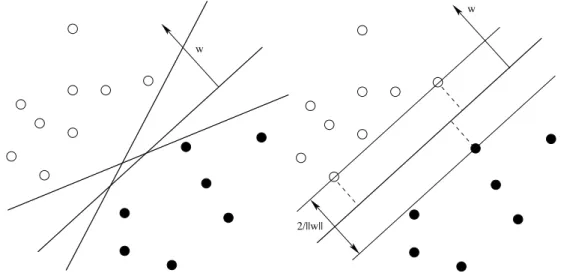
can be separated by an hyperplane with any labellings while 3 examples cannot. In this case,VC =2. . . 12 2.5 Linear decision functions for linearly separable data. (a) Solutions for
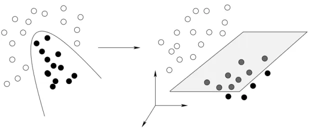
Per-ceptron. (b) The separating hyperplane that separates the data while max-imizing the margin between the two classes following the idea of Support Vector Machines. . . 14 2.6 Mapping Φ that projects 2D data onto a 3D space where the data becomes
linearly separable. . . 18 2.7 A simple decision tree with 4 decision nodes. . . 20 2.8 Curse of dimensionality. 5 examples fill more space in a 2-dimensional feature
space than in 3 dimensions. . . 21 3.1 Two possible structures for combining classifiers. . . 26 3.2 Motivations for combining several classifiers instead of only one according to
[30]. . . 27 3.3 Examples of loss functions including exponential loss (AdaBoost) and logistic
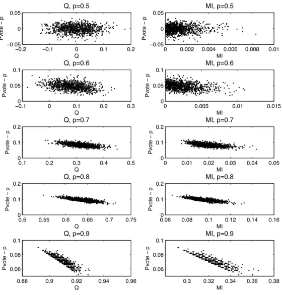
loss (LogitBoost). . . 38 4.1 Improvement of the ensemble with respect to the average individual accuracy
p={0.5,0.6,0.7,0.8,0.9}, function of 2 diversity measures. . . 44 4.2 Improvement of the ensemble w.r.t. the average individual accuracy p ∈
[0.7 0.8], function of 2 diversity measures. . . 45 4.3 Venn Diagram representing the concept of entropy and mutual information.
Mutual information can be viewed as the intersection between the marginal entropies. . . 47 4.4 Different stages of pattern recognition systems, formulated as a first order
Markov chain. . . 49 xvii
4.5 Venn Diagram representing relationships between two classifiers C1,C2 and the true class labels C. . . 51 4.6 Venn Diagram showing how to optimize classifier combination. . . 53 4.7 Diversity Accuracy dilemma. . . 54 4.8 Coupled Markov chains for 2 classifiers trained differently from the same
input data. . . 55 4.9 The similarity of 2 classifiers I(C1;C2) function of the average individual
accuracy I(C2;C)+2I(C1;C). The 2 classifiers have the same individual accuracy. 56 4.10 Graphical representation of Accuracy/Diversity dilemma. . . 56 4.11 Score behavior with synthetic class labels . . . 58 4.12 ITS in Multi-class problems. . . 59 4.13 Example of Banana distribution. 3 decision functions a re also plotted: a
decision tree, a SVM and ak−NN. . . 60 4.14 Combination accuracy and ITS for each triplet of classifiers. (a)15 SVM
with RBF kernels and (b)5 SVM with RBF kernels, 5 k−NN classifiers and 5 linear classifiers. The color of the circle is proportional the the average accuracy of the ensembles. . . 61 4.15 Example of ensemble selection withITS. Classifiers are generated on subsets
of the complete training set. Bold lines represent the 3 selected candidates. 62 4.16 Number of tests that need to be performed for classifier selection using either
exhaustive search (red) or iterative selection (blue). . . 66 4.17 Comparison between AdaBoost and its modified version based on the ITS
criterion. . . 66 4.18 Comparison between AdaBoost and its modified version based on the ITS
criterion. For each dataset, we report test error rates as function of the number of boosting iterations. . . 69 5.1 Multiple Support Vector Machines (M SVMs) . . . 72 5.2 Chromosome encoding forGAoptimization. Circles represents training
sam-ples that are used for learning each classifier. The code is 0 if none of the classifiers uses the example, 1 if only classifier 1 uses it, 4 if only classifiers 1 and 2 use it and 7 if the three classifiers have this training sample in their training set. . . 77 5.3 Illustration of the principle of Algorithm 5.2. The circles and crosses
rep-resent respectively positive and negative training samples. The number
{1,2,3}associated to each example means that the example belongs to train-ing set of the correspondtrain-ing SVM. The solid lines give the linear decision functions obtained by training 3 linear SVM using standardM SVMs tech-nique. The dashed line gives the modification of the decision functions after one iteration of KASVMs. The bold examples correspond to the ESV. The bold lines represent the ensemble decisions by voting. . . 81
List of Figures xix
5.4 Comparison between ITS-Kernel Adatron (KASVMs) and Genetic
Algo-rithms (GA) . . . 81
5.5 Comparison between M SVMsand SingleSVM on face dataset. M SVMsas defined in section 5.2 are not efficient in very low sample cases. . . 83
5.6 M SVMsin small sample cases. . . 84
6.1 An example of pre-defined line-drawing model [24]. . . 91
6.2 The shape statistic technique [16]. (a) Facial features (b)Uncertainty in shape variables when the two eyes are references, (c) Uncertainty when left eye/nose/lips are references. . . 92
6.3 Point Distributed Models [90]. A mean shape model and locations of model points. . . 94
6.4 Comparison between P CAand LDA in a two dimensional problem. [5]. . . 96
6.5 Component-based face detection [59]. a) Component templates b) Slight translation of the components c) Slight out-of-plane rotation of the head. . 97
6.6 Three variants of the like filters used in Boosting techniques. a) Haar-like filters [165], b) Extended set with rotated filters [94], c) Extended set with non adjacent regions [93] . . . 98
6.7 Gabor filters for frontal face detection [19]. . . 98
6.8 Local Binary Patterns proposed by Rodriguez et al. [132] . . . 99
6.9 An example of image of the CMU test set presented in [136]. . . 101
6.10 The criteria used in the performance evaluation proposed in [122]. . . 102
6.11 Shape of the scoring function [122] with several values of parameters α, δ andμ. . . 102
7.1 Shape of the Anisotropic Gaussian Filters. A Gaussian in one direction and its first derivative in the orthogonal direction. . . 107
7.2 Bending byr. The filter is projected onto a circle of radius r such that the y axis is a vertical tangent to that circle. . . 108
7.3 Anisotropic Gaussian filters with different rotating and bending parameters. 108 7.4 Some of the first selected base functions. . . 109
7.5 Haar-like templates. . . 109
7.6 Performance of GF and HF–based detectors on a separate test set. . . 110
7.7 ROC curves for Gaussian and Haar-like features. . . 111
7.8 Reduction of the search space by a simple cascade of Haar features. . . 111
7.9 Images that are generated from one original image taken from the BioID dataset [47]. These transformations include shifts, slight in-plane rotations, scaling and horizontal flipping. . . 112
7.10 Results on images of BANCA [4] in the complex adverse scenario. . . 114
7.11 Detection scores using the evaluation protocol [122] including the two indi-vidual scores (shift and scale) and the global score. Note that a logarithmic scale is used. . . 115
7.12 Examples of images that are considered as faces in some publications and as non faces is others. . . 116 7.13 Face detection results on some images of the MIT/CMU testset [136]. . . . 117 7.14 ROC analysis for comparing the algorithms on the MIT/CMU testset [136]. 118 8.1 Structure of the complate face detector. It comprises a cascade of 5 HF
stages followed by a mixture of 5 GF cascades. . . 125 8.2 ROC analysis for comparing the algorithms on the MIT/CMU test set [136]. 127 8.3 Comparison between 1 cascade of GF (a) and a Mixture of GF (b), both
pre-processed by 5 stages of HF. The image is taken from the CMU/MIT test set [136]. . . 129
List of Tables
4.1 Results on UCI datasets. Summary of the datasets used. Number of samples and dimensionality of the input space. We report error rates (in %) of the best single classifier and an ensemble ofK = 3 classifiers created by maximizing ITS. . . 63 4.2 Results on UCI datasets. Comparison of error rates of various methods : best
individual classifier, selection by maximalITS and selection by maximal QS. 64 4.3 Results on UCI datasets. Influence of the number of classifiers in the
ensem-ble. We report error rates (mean and standard deviation) for ensembles of K=3,5 and 7 classifiers. . . 64 5.1 Comparison of 3 classification techniques on face detection dataset. A single
SVM trained on the complete train set, multiple SVM trained by random sampling (M SVMs) and multipleSVM obtained byGAusingITS as fitness function (GASVMs). For each classifier, classification error rates are reported. 77 5.2 Comparison of various multipleSVM techniques on UCI Forest database [2].
For each technique we report the number of support vectors (#SV), the test error on a large test set and the training time in minutes. . . 82 5.3 Comparison of 3 classification techniques on several large scale datasets. A
singleSVM trained on the complete train set, mixtures ofSVM trained by random sampling and mixtures ofSVM obtained by KA-ITS. Error rates are reported for each classifier, as well as the total number of support vectors between parentheses. . . 82 7.1 Comparisons of various methods tested on the BANCA [4] database.
Re-sults are reported for the French and English parts following the evaluation protocol described in [122]. Detections with a global score larger than 0.95 are considered as correct. . . 114 7.2 Performances on the CMU/MIT test set [136]. 3 datasets configurations are
considered: Dataset 1: 155 faces, dataset2: 483 faces, Dataset 3: 507 faces. It shows the Detection rate (D.R.) and number of false alarms (F.A) for each method. . . 116
8.1 Comparisons of various methods tested on the BANCA [4] database. Re-sults are reported for the French and English parts following the evaluation protocol described in [122]. Detections with a global score larger than 0.95 are considered as correct. . . 126 8.2 Performances on the CMU/MIT test set [136]. 3 datasets configurations are
considered: Dataset 1: 155 faces, dataset2: 483 faces, Dataset 3: 507 faces. It shows the Detection rate (D.R.) and number of false alarms (F.A) for each method. . . 127 8.3 Detection speed in frames per seconds (fps) of 4 detectors. The measure is
List of Algorithms
3.1 Bagging algorithm [10] . . . 32 3.2 AdaBoost algorithm[44] . . . 34 4.1 ITS-Boost algorithm . . . 67 5.1 Kernel Adatron . . . 78 5.2 ITS - Kernel Adatron . . . 79
Abbreviations and Symbols
Mathematical notations
A, B matrices are denoted by capital letters
x,w vectors are denoted by bold lower–case letters and are column vectors
x the transposed of vector x
A the transposed of matrix A
·,· inner product operator
· norm operator
x the smallest integer grater than x
x the largest integer smaller than x
|A| determinant of a matrix A
|Ω| cardinality for a set Ω
E[·] expectation operator
List of Symbols
ANN Artificial Neural Networks
BKS Behavior Knowledge Space
DFFS Distance From Feature Space
ESV Ensemble Support Vectors
GA Genetic Algorithm
GASVMs Genetic Algorithms based Mupltiple Support Vector Machines
GF Gaussian Filters
GSVMs Gated Support Vector Machines
HF Haar-like Filters
IT Information Theory
ITA Information Theoretic Accuracy
ITD Information Theoretic Diversity
ITS Information Theoretic Score
KA Kernel Adatron
KASVMs Kernel AdaTron for Mupltiple Support Vector Machines
k−NN K-Nearest Neighbors
LDA Linear Discriminant Analysis
LBP Local Binary Patterns
M I Mutual Infirmation
M LP Multi Layer Perceptron
M SVMs Multiple Support Vector Machines
M V Majority Voting
PAC Probably Approximately Correct
P CA Principal Component Analysis
QS Q-statistics
RBF Radial Basis Functions
ROC Receiver Operating Characteristic
SM O Sequential Minimal Optimization
SVM Support Vector Machine
VC Vapnik-Chervonenkis
WITA Weighted Information Theoretic Accuracy
WITD Weighted Information Theoretic Diversity
Introduction
1
Face detection has been an active application in the field of computer vision for the last two decades, mainly because of the increasing number of potential applications in biometrics, content-based image retrieval, video conferencing or intelligent human-computer interfaces. However, detecting human faces in images can also be viewed as a very challenging machine learning task and is commonly used for the evaluating the robustness of pattern recognition techniques, from feature selection and extraction steps to classification.
The challenge of face detection in still images comes from the large variability of the face appearance due to many intra-personal and extra-personal factors, such as the modification of the face appearance with changes in illumination or head pose. Face detection can be turned into a pattern recognition task by using a sliding window that scans the image at different scales. At each position, a classifier checks the presence of a potential face.
A large number of techniques have been proposed for solving this classification problem and, one very popular classification technique for this kind of applications is to combine several classifiers to form an ensemble of classifiers. Combining classifiers was originally employed for helping the implementation of learning algorithms having large computation requirements, like Neural Networks for instance, the underlying motivation being that it is generally much easier finding several quite good classifiers than building one single very performant classifier. Then, classifier combination became a very active field in the machine learning community as it proved to be very effective in many applications, not only for re-ducing training complexity but also in terms of classification performances. Face detection is a typical problem for which combining classifiers can improve significantly the perfor-mances. On the one hand, learning a robust face model requires a huge number of training patterns, and, dealing with very large training sets presents two major drawbacks: the training procedure becomes very computationally expensive and the risk of having outliers and noisy examples is increased. Face detection can take advantage of classifier combination
techniques from four different perspectives:
• Reduce the training complexity. This step is very important in face detection as the total training time can be reduced from weeks to days;
• Reduce testing time. As most of the applications require real-time face detectors, large efforts should be put on reducing the time needed to process one single frame;
• Improve the overall performances of the system. Combining classifier can help reduc-ing number of false detections;
• Obtain sparser models. It can produce models with low storage requirements. This should be considered as a important factor in embedded systems.
Classifier combination techniques can be divided into two main categories, aggrega-tion of classifiers outputs or ensemble creaaggrega-tion techniques. On the first hand, aggregaaggrega-tion techniques dispose of a set of predefined classifiers. A combination rule then takes the clas-sification decision. The combination can be performed at the decision level (using the class labels) or at a score level (usually represented by posterior probabilities). In this catego-ry, usual applications concerns fusion of modalities (e.g. in biometrics) or combination of experts. On the second hand, ensemble creation techniques try to generate a set of classi-fiers such that their combination will be performant. Such algorithms are usually iterative procedures that grow ensembles until the expected classification performances are reached. Many studies focused on understanding why ensemble methods - even simple voting schemes - were so successfull in most of supervised classification tasks. One of the main factors that can explain this empirical observation is that, performance of complementary classifiers can be improved by aggregation, supposing that errors committed by one classifier can be corrected by the others in the team. On the contrary, combining classifier that commit errors on the same data seems to be useless. Consequently, it is commonly admitted that classifiers need to be diverse in order to improve performances compared to the best individual classifiers. In this sense, numerous diversity measures have been proposed to analyze the efficiency of classifier ensembles. However, in practice, using these diversity measures as criteria for creating good ensembles is not as successful as expected. How to efficiently use explicit measures of diversity in classifier ensembles is still an open problem in the pattern recognition community.
The work in this thesis mainly focuses on the role played by diversity in ensemble methods. In particular, we will propose an information theoretic framework for proving that diversity is, in general, not self-sufficient, but needs to be coupled carefully with the average individual accuracy of the classifiers in the team. As an illustration, we will pro-pose a complete analysis of one particular classifier combination technique: combination of Support Vector Machines. Support Vector Machines are one of the most popular dis-criminative approach of pattern recognition and is often considered as state-of-the-art in binary classification. However they present one severe drawback when facing a very large number of training examples. These classifiers become very computationally expensive to
1.1. Organization of the Thesis 3
train, mainly because of the model selection step that becomes quickly intractable. This problem can be addressed by decomposing the learning of the Support Vector Machine into several tasks with lower computational requirements. One possible solution is to split the training data into several subsets, and train in a parallel manner one Support Vector Machine on each subset. Not only does it reduce the complexity of the learning problem but, in practice, it also provides improvements in terms of classification accuracy. In fact, the implementation in a parallel structure can reduce influence of potential outliers or noise present in the training data. In this work we will propose several strategies for designing performant ensembles of Support Vector Machines, in particular based on our information theoretic framework.
1.1
Organization of the Thesis
This thesis is organized in two main parts. We will first give theoretical aspects of pattern recognition and classifier combination, in particular we will propose an information theoretic framework for combining classifiers and detail concrete example considering ensembles of support vector machines. Then, we will propose to use classifier combination techniques in a real-world application, namely frontal face detection.
Chapter 2 gives an introduction to pattern recognition from a discriminative perspec-tive and review the main classifiers used throughout the thesis: Support Vector Machines, decision trees, K-nearest neighbors, etc.
Then, chapter 3 gives a general overview of classifier combination techniques. A greedy ensemble creation technique called AdaBoost is detailed, since it will be used extensively in the face detection application.
Chapter 4 introduces the information theoretic framework for combining classifiers. We propose the so called Information Theoretic Score that measures the efficiency of an ensemble by fixing a trade-off between diversity and individual accuracies. As an illustrative use of this score, several combination techniques will be proposed.
Chapter 5 introduces new techniques for combining efficiently Support Vector Machines. The second part of the thesis will be divided into three main chapters. First, a general overview of existing face detection techniques is given in chapter 6.
Chapter 7 introduces new geometrical features that can be used to model efficiently face appearance, while chapter 8 shows how classifier combination techniques can be im-plemented successfully in a frontal face detection system.
Finally, chapter 9 will conclude by giving a short summary of the work and give the main perspectives.
1.2
Main Contributions
This thesis mainly targets the study of classifier combination and proposes, as a case study, the application to face detection. We study the concept of diversity in several classifier com-bination schemes. In particular, we propose to analyze the classifier comcom-bination problem in
an information theoretic framework and then propose solutions for tackling the limitations of pure diversity-based classifier combination techniques. We show how the new information theoretic framework can be used in the particular case of combination of Support Vector Machines. Finally we give an illustration of classifier combination techniques in a complete real-world system, namely face detection. Here is a short list of the main contributions of the present work:
• We propose an information theoretic framework to classifier combination. We will give theoretical insights justifying why an ensemble can outperform single classifier schemes. In the particular case of majority voting for combining the decisions, we show that the main challenge of optimal classifier combination is to find a trade-off between diversity in the ensemble and average individual accuracy.
• From empirical considerations we establish a link between these two contradictory quantities. We propose a new measure of the efficiency of an ensemble, the Information Theoretic Score (ITS).
• The new score is used in the context of over-production and selection of classifiers and evaluated on several common datasets.
• We then show how this framework can be extended to weighted majority voting through an example algorithm. We propose a modification of AdaBoost that takes into account the information theoretic score mentioned hereabove. AdaBoost is known for implicitly creating diversity between the hypotheses that are selected. We show that incorporating an explicit measure of diversity (through our new score) gives an algorithm that compares favorably with the standard version of AdaBoost.
• We then consider a particular classifier combination application: combination of sev-eral Support Vector Machines. This technique can be used to efficiently reduce the training complexity but we also show how it can improve classification performances by taking advantage of the classifier combination paradigm. In particular, we propose to use an on-line algorithm for training parallel Support Vector Machines jointly by taking into account the information theoretic criterion.
• Concerning the face detection application, we first present new geometrical features that efficiently model the face appearance. These new features proved to be more discriminative than the state-of-the-art features, while still being computationally efficient.
• Finally, we propose to use a classifier combination technique in the face detection application for improving both training time and classification performances. We show on standard frontal face datasets that our system compares favorably to state-of-the-art algorithms.
Part I
Theoretical Developments
Statistical Pattern
Recognition
2
2.1
Introduction
The Machine Learning field aims at developping algorithms that are able to learn by ex-perience. Learning by heart is a simple task from a mathematical perspective as it only involves memory considerations. However, machine learning refers to a more challenging task, that is learning a model from available information, such that the model will generalize to new situations. Human brain has very powerful learning capabilities, and many studies have concentrated on understanding the underlying biological phenomenon. This field of study is situated at a crossroad between various research communities such as probability and statistics, engineering, computer science, biology, medical research, signal processing, adaptive control theory, etc. In the last decades machine learning covered a wide range of applications, including automatic character recognition, speech recognition, but also med-ical diagnosis, data mining, and more recently biometrics. The large scientific research activity in this field is reflected by the publication of many books on machine learning [8, 32, 48, 57, 75, 146, 164, 167].
Pattern recognition (or classification) is the field of applications that aims at learning from a set of examples how to classify new data into a finite set of categories that are called classes. The input of a common pattern recognition system is thus an entity called pattern
(e.g. an image, an audio signal, etc.) which we aim to associate to an output class. Here are a few examples of typical pattern recognition tasks:
• Predict from various medical and demographic measurements if a patient presents risks of developing lung, prostate or breast cancers;
• Recognize automatically handwritten digits for automatically reading ZIP codes on postal envelopes;
Sensor
signal measurments features
Feature extraction
Feature selection/ Classification decision
Figure 2.1: Different stages of pattern recognition systems.
• Recognize fingerprints or faces for biometric verification purposes;
• Develop an efficient SPAM filter.
A pattern recognition system is ususally decomposed into three main steps: data acqui-sition, feature selection and extraction and finally classification. A pattern is represented by a set of measurements that should contain relevant information with respect to the structure of the object that we want to classify. The measurements can potentially be collected from a large number of sensors, thus resulting in a high dimensionality vector of measurements. The first steps in a pattern recognition system consists in processing the raw data coming from the measurements, in order to find an adequate representation of the signals. This pre-processing of the data is called feature selection and extraction. The new data called features are then given to a classifier that takes the decision. An overall view of the main stages of a pattern recognition system is shown in figure 2.1. The training examples (or training patterns) are the known instances from which we want to learn a model that can generalize to previously unseen data.
Pattern Recognition can basically be split into two categories: supervised learning and unsupervised learning.
• In supervised learning, the classes in which we want to classify the data are known a priori. Each training pattern is associated to one of these known classes (one the the 10 digits, cancer or not, SPAM or not). An example of supervised learning is face recognition. Consider the problem of recognizing the identity of of person based an image of its face. The training examples are face images from which we know the associated identities. The set of classes then corresponds to the list of known identities that are present in the training set. A robust system should be able to recognize identities of new face images for identities belonging the set of classes.
• In unsupervised learning, the true classes of the training examples is not known a priori. We seek to find the various groups of pattern present in the set of training data. The task is thus to investigate the underlying structure of the data. Clustering techniques are often used to extract the groups in the training dataset. For example, given a collection of text documents, we want to organize them according to their content similarities.
Most of the work in this thesis concentrates on supervised learning.
From a mathematical perspective, pattern recognition can be seen as a decision making process that can be summarized as follows: A given pattern x is to be assigned to one of
2.2. Theoretical Concepts of Discriminative Pattern Recognition 9
belonging to classwiis viewed as an observation drawn randomly from the class-conditional probability function p(x|wi). The optimal assignment for unknown examplesxis the class that maximizes the posterior probabilityp(wi|x) ∀i∈1, . . . , C. This principle is known as the maximum a posteriori criterion (MAP).
There are basically two different approaches for implementing the MAP principle. The first technique consists in finding directly decision functions between the classes in order to find the class that is more likely to generate the test example. This technique is known as discriminative approach. Most of the work in this thesis focus on this decision-driven strategy, that is why we will give more details in the next sections of this chapter.
The other technique tries to explicitly estimate the underlying class-conditional proba-bility densities. It is based on Bayes decision rule [157]:
p(w|x) = p(x|w).p(w)
p(x) . (2.1)
It mainly shows that posterior probabilities p(w|x) can be expressed as a function of the class conditional densities p(x|w) and the class priors p(w). In practice these class condi-tional densities are unknown and various techniques have been proposed to estimate these quantities from the training data. These techniques are called generative methods. The simplest generative method is to consider the class conditional densities to be Gaussian distributed and to estimate directly the Gaussian parameters from the training data. See [8] for a detailed overview of recent generative methods (e.g. Bayesian networks).
In the remaining of the chapter we will present the main concepts of statistical pattern recognition from a discriminative perspective.
Section 2.2 will give an overview of the main theoretical concepts of the discriminative approach to pattern recognition. Then section 2.3 gives a first example of classifier, namely Support Vector Machines. In section 2.4, we present other decision functions that will also be used throughout this thesis. Section 2.5 reviews the main principles of feature selection and extraction. Finally, section 2.6 gives more practical considerations about model selection and evaluation of the algorithms.
2.2
Theoretical Concepts of Discriminative Pattern
Recog-nition
One possible formalism of the pattern recognition task is based in statistical learning theory proposed by Vapnik [164]. In this section, we give the theoretical concepts in broad lines. The common pattern recognition task is when the output space only contains two classes. The classification problem is then a binary classification task. Nevertheless, a multi-class problem can easily be decomposed into several coupled binary problems, that is why we will only consider the binary case if not specified otherwise. Note that several applications need to cope with a very large number of classes (e.g. speech recognition where each word represents one single class) but such cases a re out of the scope of this thesis.
example to be classified belongs to one of the two classes represented by the labels y=−1 ory= 1.
Let us considerZn the set ofntraining patterns in the space Z =Rd× {−1,1}:
Zn={z1,z2, . . . ,zn}, with zi = (xi, yi)∈Z =Rd× {−1,+1}. (2.2) Each sample zi is assumed to be generated from an unknown (but fixed) probability dis-tribution function (pdf): P(x, y). For each of the training examples xi, the true class label
yi is known (supervised learning).
2.2.1 Expected Risk Minimization
The problem of learning may be expressed as an optimization problem in which one wants to find the functionf∗ from a suitably chosen set of functions F, which minimizes the risk of misclassifying new vectors drawn from the same pdf P. An example x is assigned to class +1 if f∗(x)≥0 and to the class−1 otherwise. The best function can be obtained by minimizing the so-called expected risk R onF [164]:
R(f) =EZ[L(y, f(x))] =
Z
L(y, f(x))dP(x, y), (2.3) where Lis called loss functional. The loss functional penalizes the differences between the true labelsy and the predicted ones f(x). The most commonly used loss is the binary loss (or 0/1-loss):
L(f(x), y) =
0, if f(x) =y
1, otherwise . (2.4)
It simply counts the number of misclassified examples. Other loss functionals take into ac-count the confidence that we may have for the prediction of each example. For example, the squared loss function is widely used in regression applications: L(f(x), y) = 21(f(x)−y)2. The logistic loss function is used to give a probabilistic interpretation of the output:
L(f(x), y) = log(1 + exp(−f(x)y)). More specific loss functionals will be given in sec-tion 3.5.
The optimal functionf∗ should be the one that generalizes best from training examples to new data. That is why the amount of new data that is misclassified by f∗ is called generalization error.
Unfortunately, the riskR(f) cannot be minimized directly, since the underlying distri-bution P(x, y) is unknown. Therefore, we need to find an estimate of f∗ obtained from the available information: the training set. A simple technique called induction principle consists in only computingR (equation (2.3)) on the available data. The risk is then called the empirical risk:
Remp(f, Zn) = 1 n n i=1 L(f(xi), yi). (2.5)
2.2. Theoretical Concepts of Discriminative Pattern Recognition 11
(a) Small training set (b) Solid line underfits (c) Dashed line overfits
Figure 2.2: Illustration of the overfitting and underfitting phenomena.
E[Remp(f, Zn)] = R(f) (see [164]). The empirical risk minimization consists thus in se-lecting the function: fZ∗n = arg minf∈FRemp(f, Zn). The proportion of training samples that are misclassified by the obtained function is called training error.
2.2.2 Capacity
Empirical risk minimization seems straightforward. However, it presents a major limitation known as overfitting. In order to understand the problem from a theoretical perspective, we will introduce the notion of capacity of a class of functions.
A very important step in the design of pattern recognition systems is the choice of the set of functionF in which we seek the optimal solution.
Let us consider a simple 2-dimensional problem as depicted in figure 2.2. Consider that the training set is represented by the examples in figure 2.2(a). Given only this small sample set, either the solid or the dashed hypothesis might be true, the dashed one being more complex, but also having a smaller training error.
Only when more data are available we can judge which decision function reflects best the true distribution. Let us imagine that the true distribution is in fact the one depicted in figure 2.2(b). In this case, solid line is too simple to explain the data, while the dashed line seems to generalize well. We say that the solid line underfits the data. If the true distribution is the one represented in figure 2.2(c), then the dashed line is too complex, it overfits the data. In this last case, we see that a function that minimizes the training error (dashed line in figure 2.2(a)) is not a guarantee of small generalization error.
A possible solution for avoiding overfitting is to restrict the complexity of the function class F. From a practical perspective, the main idea is that simple function that explains most of the data is preferable to a complex one. (this follows Occam’s razor principle).
More theoretically, Vapnik et al [164] showed that the solutionfZ∗n found by minimizing the empirical risk is better on the given training set Zn than on any other set drawn from
p(x, y).
In fact, the complexity of the class of functionsF plays a key role in this problem. The
capacity of a set F gives a measure of this complexity:
Definition 2.1. The capacity is the largestnsuch that there exits a set of example Znsuch that one can always find a function f ∈ F which gives the correct classification for all the
Empirical Risk Expected Risk
Capacity
Complexity of the Function Set
Figure 2.3: Illustration of the dilemma between empirical risk minimization and confidence of the function set (capacity).
n=2 d=1
d=1 n=3
Figure 2.4: Illustration of theVC dimension in a 1-dimensional feature space. 2 points can be separated by an hyperplane with any labellings while 3 examples cannot. In this
case,VC =2.
examples in Zn, for any possible labeling
In practice, controlling the capacity of decision functions is achieved by adding a regu-larization term in equation (2.5) (e.g [119, 160]).
Finding an optimal set of functions and regularization term can be viewed as a model selection step. This step is on of the most essential in order to obtain a robust decision function.
Vapnik et al [164] proposed a theory for controlling the capacity of a set of function. They define the Vapnik-Chervonenkis (VC) dimension:
Definition 2.2. Vapnik-Chervonenkis (VC) dimension of a class of functionF is the num-ber of points that can be separated for all possible labeling and using all the functions of the class F.
This VC dimension is not related to the number of parameters of the set of function but really gives a measure of the complexity. For example simple class of functions with one single parameter can produce infiniteVC.
2.3. Large Margin Classifiers 13
The main interest of VC is that it gives several formulations of upper-bounds on the expected risk. For example, the following theorem is proved in [164].
Theorem 2.1 (Vapnik et al [164]). Considering the binary loss defined in equation (2.4), for all δ >0 and f ∈F, the inequality bounding the risk:
R[f]≤Remp[f] + 1 n V C(log 2n V C −log δ 4) , (2.6)
holds with probability of at least 1−δ for n > V C.
From the bound in equation (2.6) we can distinguish two extremes:
• If the class of function F is very simple, then the squared root term vanishes but a large training error might occur.
• If F contains very complex functions, then the empirical error may be small but the regularization term may become large.
The best class of functions F is usually lies in between. Figure 2.3 gives an illustration of the trade-off between the empirical risk and the regularization term.
In fact the expected risk minimization faces a typical bias/variance dilemma. The bias comes from the choice of the set of function F. There is a bias when the optimal solution is not included into F. The variance is due to the fact that using another training set Zn
would give a different solution.
2.3
Large Margin Classifiers
In section section 2.2 we introduced the main theoretical considerations of statistical pattern recognition. Basically the goal if to find the optimal function f∗ in a class of functionsF, that minimizes the expected risk equation (2.3). In the following sections we will present several examples of decision functions that will be used widely in this thesis.
2.3.1 Introduction to Linear Machines
A first simple choice of function class F is to use simple hyperplanes for separating the two-class data. They are called linear discriminant functions, linear machines or linear classifiers. Let us consider a set of functions of the form∗:
fw,b(x) =w,x+b, (2.7)
wherewandbare the parameters of the linear function. The set of points wherefw,b(x) = 0 is called the hyperplane and the decision function is given by:
f(x) = sgn(fw,b(x)) = sgn (w,x+b). (2.8)
w
(a) Possible Perceptron solutions
2/||w||
w
(b) Hyperplane with maximal margin
Figure 2.5: Linear decision functions for linearly separable data. (a) Solutions for Perceptron. (b) The separating hyperplane that separates the data while maximizing the
margin between the two classes following the idea of Support Vector Machines.
The optimization process of the learning is to find the best function parameters w and
b. There are various motivations for using simple hyperplanes as decision functions. On the first hand it perfectly fits with Occam’s Razor principle cited in a previous section. In fact, it can be shown that for the class of hyperplanes, the VC dimension can be bounded efficiently. More details can be found in [164].
The papameters w and b can be optimized such that the number of misclassified ex-amples is minimized. This is the principle of Rosenblatt’s perceptron [135]. It considers an optimization criterion which is directly proportional to the sum of the distances of mis-classified examples to the decision boundary. A set of data is linearly separable if there exists a constant γ such that yiw,xi+b > γ for all i. The limitations of this simple mistake-driven procedure is that its convergence is only guaranteed for linearly separable data. Novikoff [107] proved that the perceptron algorithm converges after a finite number of iterations if the data set is linearly separable and the number of mistakes is bounded by
2r γ
2
, wherer=maxixi . Moreover, the perceptron algorithm stops once the training data has been correctly separated and this induces that the solution of the perceptron is not unique. This non unicity is shown in figure 2.5(a). All the candidate linear functions drawn separate perfectly the training data. However, we have no information about which one will generalize best.
Fisher introduced another criterion for separating the data but trying to separate them as much as possible (e.g [48]). This criterion is the ratio of the between-class to within-class variances. This criterion aims at finding the best separation between the classes by taking into account their respective variances. However, it is only optimal under the assumption of two normal distributions.
2.3. Large Margin Classifiers 15
2.3.2 Maximization of the Margin
A popular quantity that measures how much a linear hyperplane separates the data is the
margin. The margin is defined as the minimal distance of a sample to the decision surface. Vapnik [164] showed that the VC dimension can be bounded in terms of the margin. Linearly Separable Case
Let us first assume that the two classes are linearly separable (the non separable case will be discussed later on). The parameters w and b in equation (2.8) can be rescaled such that the closest points to the hyperplane satisfy |w,x+b|= 1. This normalization gives the so-called canonical representation of the hyperplane. Now let us call x1 and x−1 two samples of each class satisfying w,x1+b= 1 and w,x−1+b =−1. The margin ρ is given by the distance between these two points, measured perpendicular to the hyperplane:
ρ= w
w.(x1−x−1) = 2
w. (2.9)
The hyperplane perpendicular to the margin is depicted in figure 2.5(b).
From this definition, the bound linkingVC and the length of the weight vector wis:
V C ≤Λ2R2+ 1, (2.10)
where Λ ∈ R+ is a constant such that w < Λ and R is the smallest ball around the data: x< R. As we cannot directly minimize the expected risk defined in equation (2.3), we try to minimize two terms: the empirical risk in equation (2.5) and the complexity term in equation (2.6). The empirical risk is forced to be zero as we constrain b and w to linearly separate the data, and the capacity is controlled by minimizing the bound in equation (2.10). It turns out that minimizing this bound means minimizing w2.
For a fixed training set Zn, finding the optimal hyperplane (optimal in the sense of largest margin) is thus equivalent to solving a quadratic optimization problem:
min w,b 1 2w 2, (2.11) subject to: yiw,xi+b≥1, i= 1, . . . , n. (2.12) A standard approach to optimization problems with equality and inequality constraints is the Lagrange formalism [41]. The dual optimization problem is obtained by introducing the Lagrange multipliersαi>0, i= 1, . . . , n, (one for each constraint in equation (2.12)). We obtain the following Lagrangian function:
L(w, b, α) = 1 2w 2− n i=1 αi(yiw,xi+b−1). (2.13)
This function has to be minimized with respect to w, b and maximized with respect to α. The optimal saddle point equation is found at: ∂Lw = 0 and ∂Lb = 0. We obtain the following dual optimization problem:
max α n i=1 αi−1 2 n i=1 n j=1 αiαjyiyjxi,xj, (2.14) subject to: αi≥0, i= 1, . . . , n, n i=1 αiyi = 0. (2.15)
By solving this dual optimization problem, we obtain a linear decision function that only depends on dot products between training patterns:
f(x) = sign n i=1 αiyix,xi . (2.16)
We have up to now only considered the case of separable training data which corresponds to training error equal to zero. However, this might not be the optimal choice that minimizes the expected risk. This is particularly true in case of noisy data. Directly minimizing the empirical risk introduces a large risk of overfitting.
Non Linearly Separable Case
In order to find a better trade-off between empirical risk and capacity, a common strategy is to allow some training points to fall into the margin. This is done by introducing the so-called slack variables ξi that will relax the constraints defined in equation (2.12):
yiw,xi+b≥1−ξi, ξi≥0 i= 1, . . . , n. (2.17) We then add a constant C > 0 that penalizes training patterns that fall into the margin. This C controls the trade-off between empirical risk and capacity. It needs to be tuned through a model selection process. The new optimization problem:
min w,b 1 2w 2+C n i=1 ξi, (2.18)
which can be turn into another dual problem:
max α n i=1 αi−1 2 n i=1 n j=1 αiαjyiyjxi,xj, (2.19) subject to: 0≤αi≤C, i= 1, . . . , n, n i=1 αiyi = 0. (2.20)
2.3. Large Margin Classifiers 17
This formulation is known as a C-Support Vector Machine (C-SVM). Let us now analyze the decision function equation (2.16) obtained by the dual optimization problem.
A first interesting property of the SVM is given by the so-called Karush-Kuhn-Tucker conditions [163]. They show that for each training pattern:
⎧ ⎪ ⎨ ⎪ ⎩ αi = 0 ⇒ yif(xi)≥1 and ξi = 0 0< αi < C ⇒ yif(xi) = 1 and ξi = 0 αi =C ⇒ yif(xi)≤1 and ξi ≥0 (2.21)
These conditions mean that the solution equation (2.16) is sparse inα. In other words, most of the training samples are outside the margin and their corresponding αi are zero. This sparsity is one of the most attractive property of theSVM since the number of training examples the model depends on is small comparing to the size of the training set. These models are thus appealing as they have low storage requirements and usually lead to fast decision functions.
The main drawback of SVM is that finding the support vectors and their coefficients
α requires solving a quadratic optimization problem. This becomes intractable in very large scale problems. Several on-line algorithms have been proposed to find iteratively the support vectors. The two well known techniques are Kernel Adatron (KA) [148] and Sequential Minimal Optimization (SM O) [117].
2.3.3 Non Linear Classifiers in Kernel Feature Spaces
We have seen that simple decision functions are preferred in order to ovoid the problem of overfitting. However, linear decision functions are not very realistic in most applications as they present the tendency to underfit the training data. There exists various algorithms for building more complex non linear decision functions. One possibility is to use Neural Networks. An Artificial Neural Network (ANN) is an information processing paradigm that is inspired by the way biological nervous systems (human brain) process information. The non-linear decision function is obtained by merging information from a structured collection of simple decision units called neurons. See [65] for a complete review on ANN. When these decision unit are simple linear perceptrons, the algorithm is called Multi-Layer Perceptron (M LP). The weights of each perceptron are learn iteratively using feedforward or backpropagation strategies.
Another way of extending the linear decisions to non linear functions is given by the notion of kernel [1, 148, 164]. We noticed hereabove that most of real data cannot be linearly separated in the original feature space. The idea is to find a non linear mapping Φ of the data such that the examples are projected onto a potentially much higher dimensional feature space, where the data can more easily be linearly separated. The motivation of projecting data into a high dimensional feature space is that simple hyperplanes can be sufficient for separating the new data. This phenomenon is represented graphically in figure 2.6. Consequently, the mapping allows to apply the principles established of linear separable data, but in the new complex feature space.
Figure 2.6: Mapping Φ that projects 2D data onto a 3D space where the data becomes linearly separable.
Let us define the non linear mapping fromRdonto a high dimensionality Hilbert space
S:
Φ :Rd → S (2.22)
x → Φ(x).
Given this mapping Φ, all the linear techniques presented in the previous sections can be ap-plied in the new feature spaceSsimply by replacing the data{(x1, y1),(x2, y2), . . . ,(xn, yn)} by the projected data {(Φ(x1), y1),(Φ(x2), y2), . . . ,(Φ(xn), yn)}.
The new problem is then how to choose the mapping Φ. We notice that only dot products between examples are involved in the decision function given in equation (2.16). The trick is that we do not really need to explicitly know the mapping Φ, the only information we need from the feature space S is how to compute dot products in that space. A very efficient trick for computing dot products in feature spaces is to use the so-called kernel functions
[104]. A kernel function is defined as:
k:Rd×Rd → R (2.23)
x1,x2


![Figure 3.2: Motivations for combining several classifiers instead of only one according to [30].](https://thumb-us.123doks.com/thumbv2/123dok_us/414282.2547480/53.892.156.775.155.359/figure-motivations-combining-classifiers-instead-according.webp)