ABSTRACT
KENNEDY, EMESE AGNES. Swing-up and Stabilization of a Single Inverted Pendulum: Real-Time Implementation. (Under the direction of Hien Tran.)
The single inverted pendulum (SIP) system is a classic example of a nonlinear under-actuated system. Despite its simple structure, it is among the most difficult systems to control and is considered as one of the most popular benchmarks of nonlinear control theory. In the past fifty years many nonlinear methods have been proposed for the swing-up and stabilization of a self-erecting inverted pendulum, however, most of these techniques are too complex and impractical for real-time implementation.
In the first part of this dissertation, the successful real-time implementation of a nonlinear controller for the stabilization of the pendulum is discussed. The controller is based on the power series approximation to the Hamilton Jacobi Bellman (HJB) equation. The derivation of the controller is based on work that can be found in the literature, but the controller has not been used for the stabilization of an inverted pendulum before. It performs similarly to the traditional linear quadratic regulator (LQR), but has some important advantages. First, the method can stabilize the pendulum for a wider range of initial starting angle. Additionally, it can also be used with state dependent weighting matrices, Q and R, whereas the LQR problem can only handle constant values for these matrices. The use of state-dependent weighting matrices for the stabilization of an inverted pendulum in real-time has been discussed in the literature before, but only with controls that use a State Dependent Riccati Equation (SDRE) approach. The benefit of the control presented in this thesis over the SDRE controls is that it is computationally less intense and does not require the solution of complicated matrix equations at every time step. However, the control method presented cannot be used to swing-up the pendulum whereas some of the controls using the online solution of the SDRE can.
© Copyright 2015 by Emese Agnes Kennedy
Swing-up and Stabilization of a Single Inverted Pendulum: Real-Time Implementation
by
Emese Agnes Kennedy
A dissertation submitted to the Graduate Faculty of North Carolina State University
in partial fulfillment of the requirements for the Degree of
Doctor of Philosophy
Applied Mathematics
Raleigh, North Carolina
2015
APPROVED BY:
Stephen Campbell Ralph Smith
Kazufumi Ito Hien Tran
DEDICATION
BIOGRAPHY
The author was born in Budapest, Hungary, and lived in Thailand for three years where she completed high school at the International School of Bangkok. She graduated summa cum laude with Honors in Mathematics from Skidmore College in Saratoga Springs, NY, with a dual degree in Mathematics and Dance, and a minor in Computer Science. Thanks to the influence of great teachers and mentors she became interested in studying mathematics, particularly after one of her professors, Dr. Rachel Roe-Dale, asked her to participate in an undergraduate summer research program.
After finishing college, the author moved to Raleigh, NC to pursue a doctorate in Applied Mathematics at North Carolina State University. She received a MS degree in Applied Mathe-matics from NC State in 2013. Thanks to working with Dr. Ralph Smith during her first year of graduate school, the author was hired as the lab technician for the Center for Research in Scientific Computation (CRSC) at NC State. The position helped her gain valuable hands-on experience with real-time mathematical models used during several physical and biological experiments. Some of these included horizontal and vertical vibrating beams, heat transfer, retime blood pressure monitoring, and traveling waves. More importantly, this position al-lowed her the possibility of completing dissertation work with Dr. Hien Tran on the inverted pendulum.
While she enjoys working on real life mathematical applications, the author has a passion for teaching. She has taught several undergraduate mathematics classes during her graduate years, and has received two teaching awards from the University Graduate Student Association at NC State. In addition, she has completed the Certificate of Accomplishment in Teaching program. Thanks to Dr. Alina Duca, Emese became involved with teaching Calculus for Elementary Education, an inquiry based learning course developed with NSF support specifically for pre-service elementary teachers. She has also had the opportunity to regularly assist a research team led by Dr. Karen Keene in the Mathematics Education Department, which studies the mathematical sophistication of undergraduate students, and works on developing better ways students can be supported as they study mathematical concepts.
ACKNOWLEDGEMENTS
I would first like to thank my advisor, Dr. Hien Tran for believing in me and helping me achieve my goals. He has always been very supportive of me and allowed me to pursue my passion for teaching on top of my research. I would like to thank my committee members: Dr. Stephen Campbell, who has provided me with support and guidance since my first day at NC State; Dr. Ralph Smith, who has had a great influence on my graduate career since my first year, and who gave me the opportunity to work for the CRSC and connected me with Dr. Tran; and Dr. Kazufumi Ito, who agreed to serve on my committee and give me advice even before getting to know me.
I would like to thank Dr. Alina Duca and Dr. Karen Keene for letting me get involved with CELTIC, and for being wonderful mentors who truly helped me become a better teacher.
I wouldn’t have made it to graduate school without the great support and preparation I received from the math professors at Skidmore, who have become like a second family to me. I would especially like to thank Dr. Rachel Roe-Dale who pushed me to pursue a doctorate in applied math, and who has been an amazing teacher, mentor, and friend. Dr. David Vella also deserves special thanks for all his support and for being the first person who allowed me to teach a math class.
I would like to thank my friends and family for supporting me throughout my graduate journey, and for helping me get through some really difficult times.
I would like to thank my wife, Katie, for all her support and encouragement, and for keeping me sane and helping me survive.
TABLE OF CONTENTS
LIST OF TABLES . . . vii
LIST OF FIGURES . . . .viii
Chapter 1 Introduction . . . 1
1.1 Applications . . . 2
1.2 Review of Existing Control Methods . . . 2
1.3 Dissertation Outline . . . 5
Chapter 2 System Dynamics . . . 6
2.1 System Representation and Notations . . . 6
2.2 Equations of Motion . . . 7
2.2.1 Lagrange’s Method . . . 7
2.2.1.1 Potential Energy . . . 7
2.2.1.2 Kinetic Energy . . . 7
2.2.1.3 Lagrange’s Equations . . . 9
2.2.2 Converting to Voltage Input . . . 10
2.3 Model Calibration . . . 12
Chapter 3 Stabilization Control . . . 14
3.1 Problem Statement . . . 14
3.2 Power Series Based Controller . . . 15
3.2.1 Power Series Approximation . . . 16
3.2.2 Constant MatrixB . . . 19
3.2.2.1 Simulation Results: ConstantB vs. State-Dependent B . . . 19
3.2.3 Incorporation of a State-Dependent Weighting Matrix . . . 20
3.3 Stability Analysis . . . 22
3.4 Real-Time Implementation . . . 28
3.4.1 Apparatus . . . 28
3.4.2 Design Specifications . . . 28
3.5 Experimental Results . . . 29
3.5.1 Constant Weighting Matrices . . . 29
3.5.2 State-Dependent Weighting Matrix . . . 39
3.5.3 Disturbance Rejection . . . 42
Chapter 4 Swing-up Control . . . 48
4.1 Energy-based Controller . . . 48
4.1.1 Pendulum’s Energy . . . 48
4.1.2 Converting to Voltage Input . . . 49
4.1.3 Lyapunov Stability Condition . . . 50
4.1.4 Simulation Results . . . 52
4.1.5 Experimental Results . . . 53
4.2.1 Modified Lyapunov Function . . . 56
4.2.2 Simulation Results . . . 58
4.3 Incorporating Viscous Damping at the Pendulum Axis . . . 61
4.4 Simulation Results . . . 63
4.5 Experimental Results . . . 63
4.6 Summary of Swing-up Controllers . . . 64
Chapter 5 Closing Remarks . . . 67
5.1 General Conclusion . . . 67
5.2 Future Work . . . 67
REFERENCES . . . 69
APPENDICES . . . 76
Appendix A Model Parameters . . . 77
A.1 Nomenclature . . . 77
A.2 Model Parameter Values . . . 80
Appendix B MATLAB Code . . . 81
B.1 Code to Setup Parameters for the Simulink Diagrams . . . 81
B.2 Simulink Diagrams for Model Calibration . . . 86
B.3 Simulink Diagrams for Stabilization Simulation . . . 90
B.4 Simulink Diagrams and Code for Stabilizing Control . . . 92
LIST OF TABLES
Table 3.1 Summary of stabilization state response with di↵erent weighting matrices. 31 Table 3.2 Summary of control e↵ort with di↵erent weighting matrices. . . 31 Table 3.3 Summary of stabilization state response and control e↵ort for the power
series based controller with state-dependent Q vs. controllers with Q = diag(800,150,1,1). . . 40 Table 3.4 Summary of stabilization state response and control e↵ort with 1.5 pulse
LIST OF FIGURES
Figure 1.1 Inverted pendulum like systems. . . 2
Figure 2.1 Diagram of the SIP mounted on a cart. . . 6 Figure 2.2 DC Motor Electric Circuit . . . 11 Figure 2.3 Comparison of real-time data with simulated model response with and
without friction. . . 13
Figure 3.1 Stabilization controller with state-dependent B given by (3.24) versus controller with constant B given by (3.32) . . . 21 Figure 3.2 Stabilization simulation results for the power series based controller with
various initial angles, and x0= 0,↵˙0= 0,x˙0 = 0. . . 23 Figure 3.3 Stabilization simulation results for the LQR controller with various initial
angles, and x0 = 0,↵˙0 = 0,x˙0 = 0. . . 24 Figure 3.4 Stability region estimate for both the power series based controller and the
LQR controller for various initial pendulum angles and angular velocities with zero initial cart position and cart velocity. . . 25 Figure 3.5 Stability region estimate for both the power series based controller and
the LQR controller for various initial pendulum angles and cart positions with zero initial cart velocity and angular velocity. . . 25 Figure 3.6 Stability region estimate for both the power series based controller and
the LQR controller for various initial cart positions and cart velocities with zero initial pendulum angle and angular velocity. . . 26 Figure 3.7 Stability region estimate for the power series based controller for various
initial pendulum angles, angular velocities, and cart velocities with zero initial cart position. . . 26 Figure 3.8 Stability region estimate for the LQR controller for various initial
pen-dulum angles, angular velocities, and cart velocities with zero initial cart position. . . 27 Figure 3.9 Stability region estimate for the power series based controller for various
initial cart positions, pendulum angles, and angular velocities with zero initial cart velocity. . . 27 Figure 3.10 Stability region estimate for the LQR controller for various initial cart
positions, pendulum angles, and angular velocities with zero initial cart velocity. . . 28 Figure 3.11 Single inverted pendulum mounted on a Quanser IP02 servo plant. . . 29 Figure 3.12 Diagram of experimental setup. . . 29 Figure 3.13 Cart position with power series based controller vs. LQR:
Q=diag(0.75,4,0,0) and R= 0.0003. . . 32 Figure 3.14 Pendulum’s angle with power series based controller vs. LQR:
Q=diag(0.75,4,0,0) and R= 0.0003. . . 32 Figure 3.15 Cart velocity with power series based controller vs. LQR:
Figure 3.16 Pendulum’s angular velocity with power series based controller vs. LQR:
Q=diag(0.75,4,0,0) and R= 0.0003. . . 33
Figure 3.17 Control e↵ort with power series based controller vs. LQR: Q=diag(0.75,4,0,0) and R= 0.0003. . . 34
Figure 3.18 Cart position with power series based controller vs. LQR: Q=diag(5,50,0,0) and R= 0.002. . . 34
Figure 3.19 Pendulum’s angle with power series based controller vs. LQR: Q=diag(5,50,0,0) and R= 0.002. . . 35
Figure 3.20 Cart velocity with power series based controller vs. LQR: Q=diag(5,50,0,0) and R= 0.002. . . 35
Figure 3.21 Pendulum’s angular velocity with power series based controller vs. LQR: Q=diag(5,50,0,0) and R= 0.002. . . 36
Figure 3.22 Control e↵ort with power series based controller vs. LQR: Q=diag(5,50,0,0) and R= 0.002. . . 36
Figure 3.23 Cart position with power series based controller vs. LQR: Q=diag(800,150,1,1) and R= 0.1. . . 37
Figure 3.24 Pendulum’s angle with power series based controller vs. LQR: Q=diag(800,150,1,1) and R= 0.1. . . 37
Figure 3.25 Cart velocity with power series based controller vs. LQR: Q=diag(800,150,1,1) and R= 0.1. . . 38
Figure 3.26 Pendulum’s angular velocity with power series based controller vs. LQR: Q=diag(800,150,1,1) and R= 0.1. . . 38
Figure 3.27 Control e↵ort with power series based controller vs. LQR: Q=diag(800,150,1,1) and R= 0.1. . . 39
Figure 3.28 Control E↵ort with power series based controller: Q=diag(800 + 5x2,150 + 2↵2,1 + ˙x2,1 + ˙↵2) andR= 0.1 |Vm|<1.82 Volts,|Vm|avg= 0.358 Volts,R030|Vm|dt= 10.73. . . 40
Figure 3.29 State response with power series based controller: Q=diag(800 + 5x2,150 + 2↵2,1 + ˙x2,1 + ˙↵2) andR= 0.1. . . 41
Figure 3.30 Cart position response to 1.5 disturbance. . . 43
Figure 3.31 Pendulum’s angle response to 1.5 disturbance. . . 44
Figure 3.32 Cart velocity response to 1.5 disturbance. . . 45
Figure 3.33 Pendulum angular velocity response to 1.5 disturbance. . . 46
Figure 3.34 Control e↵ort with 1.5 disturbance. . . 47
Figure 4.1 Diagram representing how sg(X) is defined. The arrows indicate the di-rection of the cart’s displacement, while the number line indicates the cart’s position. . . 51
Figure 4.2 Simulated state response and control e↵ort for the energy based swing up controller given by equation (4.17) with = 4 and ⌘= 0.9. . . 54
Figure 4.3 Experimental state response and control e↵ort for the energy based swing up controller given in equation (4.17) with = 4 and ⌘= 0.9. . . 55
Figure 4.5 Simulated state response and control e↵ort for the more robust swing up controller including viscous damping at the pendulum axis. . . 65 Figure 4.6 Experimental state response and control e↵ort for the energy based swing
up controller given in equation (4.42) with 1 = 4.8, 2 = 0.6, 3 = 0.0115, and ⌘= 0.6. . . 66 Figure B.1 Main Simulink diagram used for model calibration. The SIP + IP02:
Ac-tual Plant block that communicates with the apparatus and captures the value of the states in real-time was provided by Quanser. The SIP EOM with Friction subsystem computes the simulated state response based on the nonlinear equations of motion with friction given by equations (2.33) and (2.34). The details of the subsystem are given in Figures B.2-B.4. The SIP EOM with No Friction subsystem is the same as the subsystem with friction, but the friction coefficients are ignored (i.e.Beq = 0 andBp = 0). 86
Figure B.2 SIP EOM Simulink subsystem used in the Simulink diagram given in B.1. 87 Figure B.3 x ddot EOM subsystem used in the Simulink diagram given in B.2. . . 88 Figure B.4 alpha ddot EOM subsystem used in the Simulink diagram given in B.3. . 89 Figure B.5 Main Simulink diagram used for stabilization simulation to compare the
performance of the control laws given by (3.24) and (3.32). The stabi-lizing control is computed inside a Matlab function with the command inv(R)⇤BX(u(1), u(2), u(3), u(4))0⇤(P⇤u+inv(A00 P⇤B⇤inv(R)⇤ B0)⇤(0.5⇤P⇤B2(u(1), u(2), u(3), u(4))⇤inv(R)⇤B0⇤P⇤u+ 0.5⇤P⇤B⇤
inv(R)⇤B2(u(1), u(2), u(3), u(4))0⇤P⇤u P⇤f3(u(1), u(2), u(3), u(4)))) (state-dependentB) or inv(R)⇤B0⇤P⇤u+inv(R)⇤B0⇤inv(A00 P⇤B⇤ inv(R)⇤B0)⇤P⇤f3(u(1), u(2), u(3), u(4)) (constant B). The input,u, for the block is the state vector, X. The SIP EOM with Friction subsystem computes the simulated state response based on the nonlinear equations of motion with friction given by equations (2.33) and (2.34). The details of the subsystem are given in Figures B.2-B.4 . . . 90 Figure B.6 Main Simulink diagram used for stabilization simulation. The
stabiliz-ing control is computed inside a Matlab function with the command inv(R)⇤B0 ⇤P ⇤u+inv(R)⇤B0 ⇤inv(A00 P ⇤B ⇤inv(R)⇤B0)⇤
P ⇤ f3(u(1), u(2), u(3), u(4)) (constant Q) or inv(R)⇤ B00 ⇤ P ⇤u + inv(R)⇤B0⇤inv(A00 P⇤B⇤inv(R)⇤B0)⇤(P⇤f3(u(1), u(2), u(3), u(4))+ 0.5⇤[5⇤u(1)2,0,0,0; 0,2⇤u(2)2,0,0; 0,0, u(3)2,0; 0,0,0, u(4)2]⇤u) (state-dependent Q). The input, u, for the block is the state vector, X. The SIP EOM with Friction subsystem computes the simulated state response based on the nonlinear equations of motion with friction given by equa-tions (2.33) and (2.34). The details of the subsystem are given in Figures B.2-B.4 . . . 91 Figure B.7 Main Simulink diagram to run real-time stabilization. The SIP + IP02:
Figure B.8 Code inside Embedded Matlab function block in the Simulink diagram to compute stabilizing control with constant Q based on power series expansion. . . 92 Figure B.9 Code inside Embedded Matlab function block in the Simulink diagram to
compute stabilizing control with state-dependent Q based on power series expansion. . . 93 Figure B.10 Scopes subsystem to record and plot states. . . 93 Figure B.11 Main Simulink diagram to run real-time swing-up. The SIP + IP02:
Ac-tual Plant block that communicates with the apparatus was provided by Quanser. The Mode Switching Strategy block that checks the angle of the pendulum and switches from the swing-up controller to the stabiliz-ing controller, was also provided by Quanser. The details of the Swstabiliz-ing-up Control subsystem block are given in Figure B.12 for the controller in (4.17), Figure B.15 for the controller in (4.28), and Figure B.16 for the controller in (4.42) . . . 94 Figure B.12 Simulink subsystem used to compute energy based swing-up controller in
(4.17). The details of the Compute sg subsystem block are given in Figure B.13, and the details of the Pendulum Energy subsystem block are given in Figure B.14. . . 95 Figure B.13 Simulink subsystem that computes sg. . . 96 Figure B.14 Simulink subsystem that computes the pendulum’s energy. . . 96 Figure B.15 Simulink subsystem used to compute more robust swing-up controller in
(4.28). The details of the Compute sg subsystem block are given in Figure B.13, and the details of the Pendulum Energy subsystem block are given in Figure B.14. . . 97 Figure B.16 Simulink subsystem used to compute swing-up controller with viscous
Chapter 1
Introduction
At some point in our lives almost all of us have attempted to balance a broomstick on the palm of our hand, or seen someone try to. The broomstick can be thought of as an inverted pendulum with the di↵erence being that the broomstick is free to move in a three-dimensional space while a pendulum, in this study, is mounted on a cart and can only move in a linear plane. Just like the broomstick, an inverted pendulum is a highly unstable system. Force and proper control must be appropriately applied to keep the pendulum balanced and upright.
In 1990 the International Federation of Automatic Control (IFAC) Theory Committee pub-lished a set of real world control problems that can be used to compare the benefits of new and existing control methods, called benchmark problems. One of these is the control of an inverted pendulum [23]. Despite its simple structure, the inverted pendulum is among the most difficult systems to control. This difficulty arises because the equations of motion governing the system are inherently nonlinear and because the upright position is an unstable equilibrium. Furthermore, the system is under-actuated as it has two degrees of freedom, one for the cart’s horizontal motion and one for the pendulum’s angular motion, but only the cart’s position is actuated, while the pendulum’s angular motion is indirectly controlled.
In a laboratory setting, there are two main types of Single Inverted Pendulum (SIP) systems: the rotary pendulum system, and the pendulum on a cart system. The controllers for these two systems are similar, but they have di↵erent actuator dynamics. The largest di↵erence between the two systems is that the pendulum on a cart system has a finite track length that needs to be taken into account, especially during swing-up. This dissertation only focuses on the controllers for a cart pendulum system.
without having to switch controllers [15]. The control methods presented in this dissertation accomplish the two tasks separately.
1.1
Applications
As its shape and dynamics resemble many di↵erent real world systems, the inverted pendulum has numerous applications. One of the earliest uses of an inverted pendulum was in 1844 by James Forbes in the design of a seismometer. Forbes used the fact that the upright equilibrium of the pendulum is unstable and thus very sensitive to disturbances [24]. Some other applications of the inverted pendulum include the stabilization of ships and rockets, the design of earthquake resistant buildings, and robotic arms. The inverted pendulum is also considered as an adequate model of a human standing still [76]. Figure 1.1 gives an illustration of some inverted pendulum like systems.
inverted pendulum system buildings during earthquake
humans standing segways robotic arms
rockets ships
Figure 1.1: Inverted pendulum like systems.
1.2
Review of Existing Control Methods
Below is a summary of the most popular control methods that have been implemented for an inverted pendulum, and a short discussion of the advantages and disadvantages of each method. Most of the cited references were compiled based on an extensive survey by Boubaker [15].
Fuzzy Logic and Neural Network Controllers are discussed in references [2, 78, 80]. These controllers have a simple structure and don’t require lengthy computations. They are very popular methods for both the swing-up and the stabilization of the pendulum, however, the presentation of these methods often lack the specification of the stability conditions.
Proportional-Integral-Derivative (PID) Adaptive Control is discussed in references [10, 19, 56]. This method is good for stabilizing the pendulum, but requires frequent tuning. Chang et al. discusses the implementation of a self-tuning PID controller using a Lya-punov approach in [19], but only simulation results are presented without discussion of real-time experiments.
Energy-Based Control is one of the most popular and efficient methods for swinging-up the pendulum. The global stability conditions of this approach are well proven using Lyapunov techniques. An energy based method was originally proposed by Astrom and Furuta in 1996 at the 13th IFAC World Congress [8]. Their revised paper that included the implementation of their method on a rotary pendulum was published in 2000 [9]. Later, the method was adapted for a cart-pendulum system by Angeli in [3], but without taking the finite length of the track into account. References [21, 49, 73, 83] also discuss the use of energy based controllers for the pendulum on a cart system. Control methods that consider the length of the track are presented in [20, 37].
Hybrid Control methods based on the energy approach that accomplish both the swing-up and the stabilization of the pendulum without switching controllers are presented in [4, 7, 6, 30, 74].
Sliding Mode Control is a powerful and robust control method that can be used for many practical systems that are not under actuated. In [71] a modified Van der Pol oscillator is implemented for both the swing-up and the stabilization of the pendulum, but with some performance issues. Namely, the fast switching in the implemented controller causes undesirable chattering. In [60] an aggressive sliding mode control law is presented for both the swing-up and the stabilization along with results of numerical simulations for the cart pendulum system, and real-time experimental results for the rotary pendulum system.
the cost functional. In a recent publication, Trimpe et al. proposed a self-tuning LQR approach using stochastic optimization, but the method has only been implemented in simulations and not in real-time experiments [77].
Linear Quadratic Gaussian (LQG) is a controller that combines LQR with a Kalman Filter to improve disturbance rejection. This method was implemented by Eide et al. in [25] during the balance of an inverted pendulum mobile robot, however, they found that the LQR produced better response when compared to the LQG approach.
Approximate Linearization is a method of finding a nonlinear change of coordinates for a nonlinear system to construct a linear approximation of the plant dynamics accurate to second or higher order. Starting with the work of Krener [41, 42, 43], many variants of this approach have been suggested [38, 40]. The algorithm presented in [41] was implemented for the stabilization of a rotary pendulum by Sugie and Fujimoto [75]. They showed through experiments that the method enlarges the stability region. Using the ideas in [42] and [40], Ohsumi and Izumikawa implemented in real-time a control method that can be used for both the swing-up and stabilization of an inverted pendulum on a cart [57]. Based on Krener’s approach, Guzzella and Isodori developed a simpler and more direct method to calculate the quantities involved [31]. This algorithm was implemented for the stabilization of a cart-pendulum system by Renou and Saydy [69]. Their simulation and experimental results show a sight improvement in the system’s transient response, but a reduced region of stability when compared to the LQR control method. In [39], Ingram et al. present the successful real-time implementation of a modified approach using an algorithm designed for feedback linearizable systems. Their technique works for both the swing-up and stabilization of an inverted pendulum on a cart. They consider both the finite track length, and the restriction on the maximum voltage input, but they do not take the e↵ects of friction into account.
State-Dependent Riccati Equation (SDRE) based controller has been used for the stabi-lization of the pendulum in simulations in [37, 72]. In [22], Dang and Lewis present the successful real-time implementation of a SDRE based controller for both the swing-up and the stabilization. The drawback of this method is that it is computationally very intense as it requires the solution of complicated state-dependent Riccati equations at every time step.
implementation for the stabilization of the pendulum [18, 17]. They have also showed that disregarding friction produces oscillatory behavior during stabilization.
1.3
Dissertation Outline
In the past sixty years many nonlinear methods have been proposed for the swing-up and stabilization of a single inverted pendulum, however, many of these techniques are too complex and impractical for real-time implementation [15]. This dissertation focuses on the real-time implementation of practical control methods for both the swing-up and the stabilization of an inverted pendulum.
In Chapter 2, the dynamics of the inverted pendulum system are discussed, including mod-eling conventions and the derivation of the nonlinear equations of motion.
Chapter 3 focuses on the adaptation of a power series approximation based control method for the stabilization of the pendulum. This control method was first proposed by Garrard in [26, 27, 28], but it has not been implemented for an inverted pendulum before. The controller performs similarly to the traditional linear quadratic regulator, but has some important advan-tages. One of the advantages is that the method can stabilize the pendulum for a wider range of initial starting angle. It can also be used with state dependent weighting matrices whereas the LQR problem can only handle constant values forQand R. The use of a state-dependent ma-trix,Q, is also discussed in this chapter. We present both simulation and real-time experimental results implemented in MATLAB Simulink.
In Chapter 4, we use the technique originally proposed by Astrom and Furuta [8, 9] to derive a modified energy based swing-up controller using Lyapunov functions. During the derivation, all e↵ort has been made to use a more complex dynamical model for the SIP system than the simplified model that is most commonly used. We consider the electrodynamics of the DC motor that drives the cart, and incorporate viscous damping friction as seen at the motor pinion. Furthermore, we use a new method to account for the limitation of having a cart-pendulum system with a finite track length. Two modifications to the controller are also discussed to make the method more appropriate for real-time implementation. One of the modifications improves robustness using a modified Lyapunov function for the derivation, while the other one incorporates viscous damping as seen at the pendulum axis. We present both simulation and real-time experimental results implemented in MATLAB Simulink.
Chapter 2
System Dynamics
2.1
System Representation and Notations
Figure 2.1 shows a diagram of the Single Inverted Pendulum (SIP) mounted on a cart. The nomenclature corresponding to the system is given in Appendix A.1. The positive sense of rotation is defined to be counterclockwise, when facing the cart. The perfectly vertical upward pointing position of the inverted pendulum corresponds to the zero angle. The positive direction of the cart’s displacement is to the right when facing the cart, as indicated by the Cartesian frame of coordinates presented in Figure 2.1.
0 x
y
Fc >0
M
x
yp
Mp
xp
`p
↵(t)
˙
↵(t)>0
2.2
Equations of Motion
2.2.1 Lagrange’s Method
We will use Lagrange’s energy method to derive the dynamic model of the system. In this approach, we consider the driving force, Fc, generated by the DC motor acting on the cart
through the motor pinion as the single input. To carry out Lagrange’s method, first we need to determine the Lagrangian of the system through the calculation of the system’s total potential and kinetic energies.
2.2.1.1 Potential Energy
The total potential energy, VT, in a system is given by the amount of energy that the system
has due to some kind of work being, or having been, done to it. It is usually caused by its vertical displacement (gravitational potential energy) from normality or by a spring-related sort of displacement (elastic potential energy). For the SIP system, the potential energy is only due to gravity. Since the carts linear motion is horizontal with no vertical displacement, the total potential energy is fully described by the pendulum’s gravitational potential energy,
VT =Mpgyp =Mpg`pcos(↵(t)). (2.1)
2.2.1.2 Kinetic Energy
Next, we will determine the system’s total kinetic energy,KT. The kinetic energy measures the
amount of energy in a system due to its motion. For the SIP system, the total kinetic energy is given by the sum of the translational and rotational kinetic energies of both the cart and its mounted inverted pendulum.
The translational kinetic energy of the motorized cart, Kct, is
Kct=
1 2Mx˙(t)
2. (2.2)
The cart’s rotational kinetic energy,Kcr, is due to the movement of the DC motor’s output
shaft, and is given by
Kcr =
1 2Jm!
2
m. (2.3)
Using the DC motor and planetary gear head technical specification sheets provided in [63] we can express the motor shaft angular velocity,!m, in terms of the angular velocity of the motor
pinion, !, as
By considering the rack and pinion and the gearbox mechanism, we can rewrite (2.4) in terms of the cart’s velocity as
Kg!=
Kgx˙(t)
rmp
. (2.5)
Substituting equations (2.4) and (2.5) into (2.3), we can express the rotational kinetic energy of the cart as
Kcr =
JmKg2x˙(t)2
2r2 mp
. (2.6)
The mass of the single inverted pendulum is assumed to be concentrated at its Center Of Gravity (COG), and the pendulum’s COG’s velocity, vCOGis given by
vCOG=
q ˙
xp(t)2+ ˙yp(t)2. (2.7)
According to the reference frame definition presented in Figure 2.1, the absolute Cartesian coordinates of the pendulum’s center of gravity are
xp(t) =x(t) `psin(↵(t)) and yp(t) =`pcos(↵(t)). (2.8)
After di↵erentiating (2.8), we can rewrite (2.7) as
vCOG=
q ˙
x(t)2 2`
pcos(↵(t)) ˙x(t) ˙↵(t) +`2p↵˙(t)2 (2.9)
Therefore, the pendulum’s transitional kinetic energy,Kpt, can be expressed as a function of its
center of gravity’s linear velocity,
Kpt= 1
2Mpv 2 COG=
1
2Mp x˙(t) 2 2`
pcos(↵(t)) ˙x(t) ˙↵(t) +`2p↵˙(t)2 . (2.10)
Furthermore, the pendulum’s rotational kinetic energy, Kpr, at its COG is given by
Kpr =
1 2Ip↵˙(t)
2, (2.11)
where the pendulum’s moment of inertia at its COG,Ip is
Ip =
Z `p
`p
r2Mp 2`p
dr= 1 3Mp`
2
p. (2.12)
Therefore, the total kinetic energy,KT, of the system is the sum of the four individual kinetic
the system’s total kinetic energy, can be written as
KT =
1
2 M+Mp+ JmKg2
r2 mp
! ˙
x(t)2 Mp`pcos(↵(t)) ˙x(t) ˙↵(t) +
2 3Mp`
2
p↵˙(t)2. (2.13)
2.2.1.3 Lagrange’s Equations
The Lagrangian,L, is given by the di↵erence of the total kinetic energy and the total potential energy,
L=KT VT. (2.14)
Substituting (2.1) and (2.13) into (2.14) yields
L= 1
2 M+Mp+ JmKg2
r2 mp
! ˙
x(t)2 Mp`pcos(↵(t)) ˙x(t) ˙↵(t) +2
3Mp` 2
p↵˙(t)2 Mpg`pcos(↵(t)).
(2.15) By definition, the two Lagrange’s equations for our system are
@2 @t@x˙L
@
@xL=Fc Beqx˙(t) (2.16)
and
@2 @t@↵˙L
@
@↵L= Bp↵˙(t), (2.17)
whereBeq is the equivalent viscous damping coefficient as seen at the motor pinion, andBp is
the equivalent viscous damping coefficient as seen at the pendulum axis [67]. Thus, equations (2.16) and (2.17) account for friction in the form of equivalent viscous damping, however, it should be noted that in the development of the current model the (nonlinear) Coulomb friction applied to the cart, and the force on the cart due to the pendulum’s action have been neglected. Using (2.15), the left-hand side of (2.16) can be expressed as
@2
@t@x˙L
@ @xL=
@ @t
M+Mp+
JmKg2
r2 mp
! ˙
x(t) Mp`pcos(↵(t)) ˙↵(t)
!
(2.18)
= M +Mp+
JmKg2
r2 mp
! ¨
x(t) +Mp`psin(↵(t)) ˙↵(t)2 Mp`pcos(↵(t))¨↵(t).
Similarly, the left-hand side of (2.17) can be written as
@2
@t@↵˙L
@ @↵L=
@ @t
✓
Mp`pcos(↵(t)) ˙x(t) +
4 3Mp`
2 p↵˙(t)
◆
Mp`pgsin(↵(t)) (2.20)
= Mp`pcos(↵(t))¨x(t) +
4 3Mp`
2
p↵¨(t) Mp`pgsin(↵(t)). (2.21)
Then, using (2.19) in equation (2.16) gives
M +Mp+
JmKg2
r2 mp
! ¨
x(t) +Mp`psin(↵(t)) ˙↵(t)2 Mp`pcos(↵(t))¨↵(t) =Fc Beqx˙(t), (2.22)
and using (2.21) in equation (2.17) gives
Mp`pcos(↵(t))¨x(t) +4
3Mp` 2
p↵¨(t) Mp`pgsin(↵(t)) = Bp↵˙(t). (2.23)
Solving Equations (2.22) and (2.23) for the second-order time derivatives ofx and↵ results in the two nonlinear equations
¨
x(t) = 3r 2
mpBpcos(↵(t)) ˙↵(t)
`pD(↵)
4Mp`pr2mpsin(↵(t)) ˙↵(t)2
D(↵)
4rmp2 Beqx˙(t)
D(↵)
+ 3Mpr 2
mpgcos(↵(t)) sin(↵(t))
D(↵) +
4r2 mpFc
D(↵)
(2.24)
and
¨
↵(t) = 3(M r 2
mp+Mprmp2 +JmKg2)Bp↵˙(t)
Mp`2pD(↵)
3Mprmp2 cos(↵(t)) sin(↵(t)) ˙↵(t)2
D(↵) 3r2
mpBeqcos(↵(t)) ˙x
`pD(↵)
+ 3(M r 2
mp+Mpr2mp+JmKg2)gsin(↵(t))
`pD(↵)
+ 3r 2
mpcos(↵(t))Fc
`pD(↵)
, (2.25)
where D(↵) = 4M r2mp+Mpr2mp+ 4JmKg2 + 3Mprmp2 sin2(↵(t)). Equations (2.24) and (2.25)
represent the Equations Of Motion (EOM) of the SIP system.
2.2.2 Converting to Voltage Input
In our real-time implementation the system’s input is equal to the cart’s DC motor voltage,Vm,
circuit of a standard DC motor given in Figure 2.2. The driving force, Fc can be expressed as
Fc =
KgTm
rmp
. (2.26)
By Kirchho↵’s voltage law, the directed sum of the electrical potential di↵erences around any
M
Im
Vm
Rm Lm
Tm,!m
Eemf
Figure 2.2: DC Motor Electric Circuit
closed circuit is zero, which means that for our system
Vm RmIm Lm
✓ d dtIm
◆
Eemf = 0. (2.27)
Since Lm<< Rm, we can disregard the motor inductance and obtain
Im=
Vm Eemf
Rm
. (2.28)
The back-electromotive-force (EMF) voltage created by the the motor is proportional to the motor shaft velocity (i. e., Eemf =Km!m), so we can rewrite (2.28) as
Im =
Vm Km!m
Rm
, (2.29)
whereKm is the back-EMF constant. Furthermore, the torque,Tm, generated by the DC motor
can be expressed as
Substituting equations (2.29) and (2.30) into equation (2.26) leads to
Fc =
KgKt(Vm Km!m)
Rmrmp
. (2.31)
Using equations (2.4) and (2.5) in (2.31), and rearranging leads to
Fc =
Kg2KtKmx˙(t)
Rmr2mp
+KgKtVm Rmrmp
. (2.32)
Utilizing (2.32) to convert the driving force to voltage input, we can rewrite the EOM given in (2.24) and (2.25) as
¨
x(t) = 3r 2
mpBpcos(↵(t)) ˙↵(t)
`pD(↵)
4Mp`pr2mpsin(↵(t)) ˙↵(t)2
D(↵)
4(Rmr2mpBeq+Kg2KtKm) ˙x(t)
RmD(↵)
+3Mpr 2
mpgcos(↵(t)) sin(↵(t))
D(↵) +
4rmpKgKtVm
RmD(↵)
(2.33)
and
¨
↵(t) = 3(M r 2
mp+Mpr2mp+JmKg2)Bp↵˙(t)
Mp`2pD(↵)
3Mpr2mpcos(↵(t)) sin(↵(t)) ˙↵(t)2
D(↵) 3(Rmr2mpBeq+Kg2KtKm) cos(↵(t)) ˙x
Rm`pD(↵)
+3(M r 2
mp+Mpr2mp+JmKg2)gsin(↵(t))
`pD(↵)
+ 3rmpKgKtcos(↵(t))Vm Rm`pD(↵)
.
(2.34)
2.3
Model Calibration
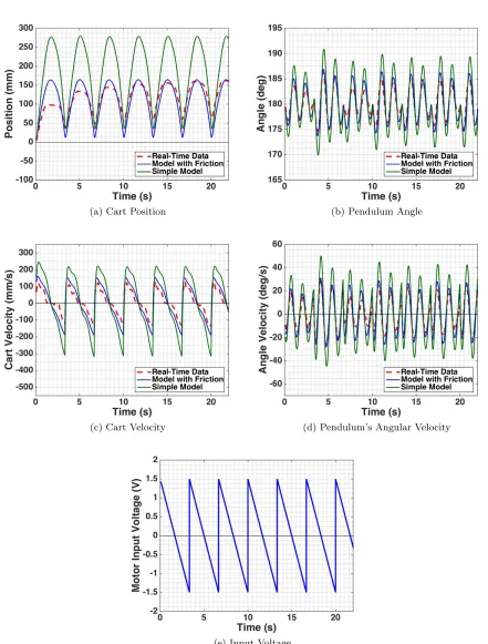
Using the Simulink diagrams in Appendix B.2, we compare the real-time states with the states obtained by our model in response to the same voltage input. The parameter values used during the simulation are given in Appendix A.2. We test the performance of our model both with and without the viscous damping friction terms,BeqandBp. The voltage input for the experiment is
(a) Cart Position (b) Pendulum Angle
(c) Cart Velocity (d) Pendulum’s Angular Velocity
(e) Input Voltage
Chapter 3
Stabilization Control
3.1
Problem Statement
Based on the Equations of Motion, (2.33) and (2.34), the state-space representation of our system has the form
d
dtX(t) =f(X(t)) +B(X(t))u(t) (3.1) where X, the system’s state vector is given by XT(t) = [x(t),↵(t),x˙(t),↵˙(t)] = [x1, x2, x3, x4], and the input u is set to equal the input voltage of the cart’s DC motor, i.e. u = Vm. The
nonlinear function f(X) can be expressed as
f(X) = 2 6 6 6 6 6 6 4
0 0 1 0
0 0 0 1
0 0 a33 a34 0 0 a43 a44 3 7 7 7 7 7 7 5 2 6 6 6 6 6 6 4 x1 x2 x3 x4 3 7 7 7 7 7 7 5 + 2 6 6 6 6 6 6 4 0 0
3Mpr2mpgcos(x2) sin(x2) D(x2)
3(M r2
mp+Mpr2mp+JmKg2)gsin(x2) `pD(x2)
3 7 7 7 7 7 7 5 (3.2) where
a33=
4(Rmr2mpBeq+Kg2KtKm)
RmD(x2)
a43=
3(Rmr2mpBeq+Kg2KtKm) cos(x2)
Rm`pD(x2)
a34=
3r2mpBpcos(x2) + 4Mp`2prmp2 sin(x2)x4
`pD(x2)
a44=
3(M r2
mp+Mpr2mp+JmKg2)Bp+ 3Mp2`2pr2mpcos(x2) sin(x2)x4
Mp`2pD(x2)
B(X(t)), in Equation (3.1) is given by
B(X(t)) = 2 6 6 6 6 6 6 4 0 0 4rmpKgKt
RmD(x2) 3rmpKgKtcos(x2)
`pRmD(x2) 3 7 7 7 7 7 7 5 . (3.3)
Now, consider the cost functional
J(X0, u) = Z 1
0
XTQX +Ru2 dt, (3.4)
where Q is a given constant-valued 4⇥4 symmetric positive-semidefinite matrix and R is a positive scalar. In the case of starting and balancing the inverted pendulum in the upright position, the optimal control problem is to find a state feedback controlu⇤(X) which minimizes the cost (3.4) for the initial conditionX0T = [0,0,0,0].
The optimal feedback control for the system in (3.1) with cost (3.4) has the form
u⇤(X) = 1 2R
1BT(X)S
X(X), (3.5)
where the function S is the solution to the Hamilton-Jacobi-Bellman (HJB) equation
SXT(X)f(X) 1 4S
T
X(X)B(X)R 1BT(X)SX(X) +XTQX = 0, (3.6)
and SX represents the Jacobian of S with respect to the states.
3.2
Power Series Based Controller
3.2.1 Power Series Approximation
As has been done by Garrard and others in references [26, 28, 27], the solution of the HJB equation can be numerically approximated using its power series expansion
S(X) =
1
X
n=0
Sn(X), (3.7)
where eachSnis a scalar polynomial containing all possible combinations of products of the state
elements with a total order ofn+2. Similarly, the nonlinear functionf(X) can be approximated by
f(X) =A0X+
1
X
n=2
fn(X), (3.8)
where eachfnis a function vector with a scalar polynomial containing all possible combinations
of products of the state elements with a total order ofn in every row. In our implementation, the power series of f was calculated using the MATLAB function taylor from the Symbolic Math Toolbox. Here, A0 represents the linearization of f(X) around the upright position (i.e.
XT = [0; 0; 0; 0]) and is given by
A0 = 2 6 6 6 6 6 6 4
0 0 1 0
0 0 0 1
0 3Mpr2mpg D
4(Rmr2mpBeq+Kg2KtKm) RmD
3r2 mpBp `pD
0 3(M rmp2 +Mpr2mp+JmKg2)g `pD
3(Rmr2mpBeq+Kg2KtKm) Rm`pD
3(M r2
mp+Mprmp2 +JmKg2)Bp Mp`2
pD 3 7 7 7 7 7 7 5 ⇡ 2 6 6 6 6 6 6 4
0 0 1 0
0 0 0 1
0 1.4967 11.6073 0.004821 0 25.6815 26.3643 0.08273
3 7 7 7 7 7 7 5 , (3.9)
where D= 4M r2mp+M prmp2 + 4JmKg2. Furthermore, the state-dependent matrix, B(X), can
be approximated by
B(X) =
1
X
n=0
Bn(X), (3.10)
where each Bn is a 4⇥1 vector with a scalar polynomial containing all possible combinations
is given by B = 2 6 6 6 6 6 6 4 0 0 4rmpKgKt Rm(4M r2
mp+Mpr2mp+4JmKg2) 3rmpKgKt
`pRm(4M r2
mp+Mpr2mp+4JmK2g) 3 7 7 7 7 7 7 5 ⇡ 2 6 6 6 6 6 6 4 0 0
1.52441 3.46248 3 7 7 7 7 7 7 5 . (3.11)
The matrices in (3.9) and (3.11) were evaluated using the parameter values from Appendix A.2. The expansions (3.7), (3.8), and (3.10) can be substituted into the HJB equation (3.6) to yield
"1 X
n=0 (Sn)TX
# " A0X+
1 X n=2 fn # 1 4 " 1 X n=0 (Sn)TX
# " 1 X n=0 Bn # R 1 "1 X n=0
BnT # "1
X
n=0 (Sn)X
#
+XTQX = 0. (3.12) We can separate out powers of the states to obtain a series of equations,
(S0)TXA0X 1 4(S0)
T
XB0R 1B0T(S0)X +XTQX = 0, (3.13)
(S1)TXA0X 1 4(S1)
T
XB0R 1B0T(S0)X
1 4(S0)
T
XB0R 1B0T(S1)X
1 4(S0)
T
XB1R 1B0T(S0)X
1 4(S0)
T
XB0R 1B1T(S0)X+ (S0)TXf2(X) = 0 (3.14)
(Sn)TXA0X 1 4
n
X
k=0 n kX
j=0 n k jX
i=0 ⇥
(Sk)TXBjR 1BiT(Sn k j i)X
⇤ + n 1 X k=0 ⇥
(Sk)TXfn+1 k(X)
⇤ = 0,
(3.15) wheren= 2,3,4, . . .. The solution of equation (3.13) is
S0(X) =XTP X, (3.16)
where the symmetric positive-definite matrix,P, solves the Algebraic Riccati Equation (ARE)
P A0+AT0P P B0R 1BT0P +Q= 0. (3.17)
Note that using (3.16) in (3.5) results in the traditional (LQR) control. The theories for the LQR problem have been well-established, and multiple stable and robust algorithms for solving (3.17) have already been developed and are well documented in the literature and in textbooks [13, 48]. It is possible to solve equations (3.14)-(3.15) for Sn, n = 1,2,3, . . ., however, this
finding (S1)X and obtaining a quadratic type control. Instead of the polynomial representation,
we may use the solution of (3.13) and make the substitution (S0)X = 2P X in equation (3.14)
to obtain
(S1)TXA0X 1 4(S1)
T
XB0R 1B0T(2P X) 1 4(2X
TP)B
0R 1B0T(S1)X
1 4(2X
TP)B
1R 1B0T(2P X) 1
4(2X
TP)B
0R 1B1T(2P X) + (2XTP)f2(X) = 0. (3.18)
This can be rearranged to yield
XT⇥AT0(S1)X P B0R 1B0T(S1)X P B1R 1B0TP X P B0R 1B1TP X+ 2P f2(X) ⇤
= 0, (3.19) which is satisfied when
(S1)X = AT0 P B0R 1B0T 1
P B1R 1BT0P X +P B0R 1B1TP X 2P f2(X) . (3.20)
Equation (3.30) along with the (S0)X term give a quadratic feedback control law of the form
u⇤(X) = R 1B0T
P X+ AT0 P B0R 1B0T
1✓1
2P B1R
1BT 0P X+
1
2P B0R
1BT
1P X P f2(X)
◆
.
(3.21)
The series expansion off(X) in our case doesn’t contain any quadratic terms (i.e.f2(X) = 0), and B1 = 0, so (3.14) is trivially solved by S1 = 0. In this case, by [14], equation (3.15) for
n= 2 will be of the form
(S2)TXA0X 1 4(S2)
T
XB0R 1B0T(S0)X
1 4(S0)
T
XB0R 1B0T(S2)X
1 4(S0)
T
XB2R 1B0T(S0)X
1 4(S0)
T
XB0R 1B2T(S0)X+ (S0)TXf3(X) = 0 (3.22)
which is exactly the same form as (3.14) except that S1 is replaced be S2, B1 is replaced by
B2, andf2 is replaced by f3. Thus, the solution is comparable to that of (3.14), with
(S2)X = AT0 P B0R 1B0T 1
P B2R 1BT0P X +P B0R 1B2TP X 2P f3(X) , (3.23)
resulting in a feedback control of the form
u⇤(X) = R 1B0T
P X+ AT0 P B0R 1B0T
1✓1
2P B2R
1BT 0P X+
1
2P B0R
1BT
2P X P f3(X)
◆
.
3.2.2 Constant Matrix B
The previously derived control law given by (3.24) can be simplified by replacing the state-dependent matrixB(X) by its linearization,B0 in the state-space representation of our system given by (3.1). Doing this yields the state-space representation in the form
d
dtX(t) =f(X(t)) +B0u(t) (3.25a)
X(0) =X0. (3.25b)
Then, equation (3.12) becomes "1
X
n=0 (Sn)TX
# " A0X+
1
X
n=2
fn(X)
# 1 4 "1 X n=0 (Sn)TX
#
B0R 1BT0 "1
X
n=0 (Sn)X
#
+XTQX = 0. (3.26)
Separating out powers of the states modifies the system of equations in (3.13)-(3.15) to
(S0)TXA0X 1 4(S0)
T
XB0R 1B0T(S0)X +XTQX = 0, (3.27)
(S1)TXA0X 1 4(S1)
T
XB0R 1B0T(S0)X
1 4(S0)
T
XB0R 1B0T(S1)X + (S0)TXf2(X) = 0, (3.28)
(Sn)TXA0X 1 4 n X k=0 ⇥
(Sk)TXB0R 1B0T(Sn k)X
⇤ + n 1 X k=0 ⇥
(Sk)TXfn+1 k(X)
⇤
= 0, (3.29)
wheren= 2,3,4, . . .. The solution to (3.28) is
(S1)X = 2(AT0 P B0R 1B0T) 1P f2(X), (3.30)
which yields the quadratic feedback control law of the form
u⇤(X) = R 1BT0 ⇥P X (A0T P B0R 1B0T) 1P f2(X) ⇤
. (3.31)
As before, since for our model f2(X) = 0, we replace S1 by S2, and f2 by f3 to obtain the control law
u⇤(X) = R 1BT0 ⇥P X (A0T P B0R 1B0T) 1P f3(X) ⇤
. (3.32)
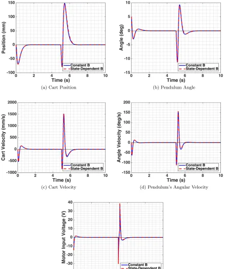
3.2.2.1 Simulation Results: Constant B vs. State-Dependent B
we introduce a 10 angular disturbance. The simulation results are given Figure 3.1. It can be seen that the two controllers perform very similarly near the upright position, so in future implementations we will use the simpler controller with constant B given by (3.32).
3.2.3 Incorporation of a State-Dependent Weighting Matrix
The performance of the controller greatly depends on the selection of the constant valued weighting matrices,Q andR, in the cost function (3.4). Finding the right values that will lead to the desired performance requires careful tuning that can be very time consuming. Changing these matrices from constant to state-dependent can not only improve the performance of the controller, but can also shorten the time required for tuning. The above derivation can be adapted to incorporate a state-dependent matrix,Q(X), into the cost function. To do this, first we need to expandQ(X) as a power series
Q(X) =
1
X
n=0
Qn(X), (3.33)
where the entries in each Qn are scalar polynomials containing all possible combinations of
products of the state elements with a total order ofn. ReplacingQby the power series ofQ(X) in equation (3.26) and separating out powers of the states modifies the system of equations in (3.27)-(3.29) to
(S0)TXA0X 1 4(S0)
T
XB0R 1B0T(S0)X +XTQ0X= 0, (3.34)
(S1)TXA0X 1 4(S1)
T
XB0R 1B0T(S0)X
1 4(S0)
T
XB0R 1B0T(S1)X + (S0)TXf2(X) +XTQ1X= 0, (3.35)
(Sn)TXA0X 1 4 n X k=0 ⇥
(Sk)TXB0R 1B0T(Sn k)X⇤+ n 1 X
k=0 ⇥
(Sk)TXfn+1 k(X)
⇤
+XTQnX= 0,
(3.36)
wheren= 2,3,4, . . .. The solution to (3.35) is
(S1)X = (AT0 P B0R 1B0T) 1(2P f2(X) +Q1X), (3.37)
which yields the feedback control law
u⇤(X) = R 1B0T
P X (AT0 P B0R 1BT0) 1 ✓
P f2(X) +1 2Q1X
◆
(a) Cart Position (b) Pendulum Angle
(c) Cart Velocity (d) Pendulum’s Angular Velocity
(e) Input Voltage
Since for our model f2(X) = 0, we will defineQ so that Q1 = 0 to make sure that (3.35) can be solved trivially byS1 = 0. As before, in this case we can replaceQ1 byQ2,S1 byS2, andf2 by f3 to obtain the the control law
u⇤(X) = R 1B0T
P X (AT0 P B0R 1BT0) 1 ✓
P f3(X) + 1 2Q2X
◆
. (3.39)
3.3
Stability Analysis
Using the Simulink diagram provided in Figure B.6 with various initial states, we can estimate the stability region for both the power series controller and the LQR controller. The parameters in the Simulink diagrams are initialized using the Matlab code provided in Appendix B.1.
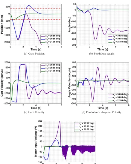
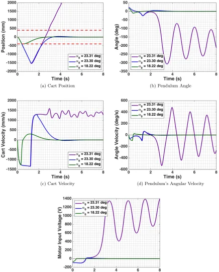
First, we only consider di↵erent initial pendulum angles and make the other initial states zero. We repeat the simulation several times with di↵erent initial angles to find the first angle where each of the controllers is able to stabilize the pendulum. This angle for the power series based controller is ↵0 = 30.85 , while for the LQR controller it is ↵0 = 23.30 . Since we have a finite track length, we continue repeating the simulation until we find the first initial angle where each of the controllers is able to stabilize the pendulum and the position of the cart stays within the track (i.e.|x|<400 mm). The first such angle for the power series based controller is ↵0 = 21.08 , while for the LQR controller it is ↵0 = 18.22 . The simulated state responses and control e↵ort for these angles of interest are given in Figure 3.2 for the power series based controller and Figure 3.3 for the LQR controller. The red dashed lines in Figures 3.2a and 3.3a indicate the end of the track.
To get a better estimate of the stability region for the power series controller and the LQR controller, we repeat the simulations with various initial conditions for two of the states while keeping the initial condition for the other two states zero. The stability region estimates for initial conditions 180 ↵0 180 , 590 /s↵˙0 590 /s,x0 = 0, and ˙x0 = 0 are given in Figure 3.4, for initial conditions 180 ↵0 180 , 390 mm x0 390 mm, ˙x0 = 0, and ˙↵0 = 0 are given in Figure 3.5, and for initial conditions 390 mm x0 390 mm, 1000 mm/s x˙0 1000 mm/s, ↵0 = 0, and ˙↵0 = 0 are given in Figure 3.6. The range on the velocities was selected based on the values possible by the apparatus we use for real-time implementation, while the range on the cart’s position was selected to be within the length of the track. For all three cases, the stability region of the power series controller is bigger than the stability region of the LQR controller.
(a) Cart Position (b) Pendulum Angle
(c) Cart Velocity (d) Pendulum’s Angular Velocity
(e) Control E↵ort
(a) Cart Position (b) Pendulum Angle
(c) Cart Velocity (d) Pendulum’s Angular Velocity
(e) Control E↵ort
Figure 3.4: Stability region estimate for both the power series based controller and the LQR controller for various initial pendulum angles and angular velocities with zero initial cart position and cart
velocity.
Figure 3.5: Stability region estimate for both the power series based controller and the LQR controller for various initial pendulum angles and cart positions with zero initial cart velocity and angular
Figure 3.6: Stability region estimate for both the power series based controller and the LQR controller for various initial cart positions and cart velocities with zero initial pendulum angle and angular
velocity.
mm/s, andx0= 0 is given in Figure 3.7 for the power series based controller and in Figure 3.8 for the LQR controller. The stability region estimate for initial conditions 180 ↵0 180 , 590 /s↵˙0 590 /s, 390 mmx0 390 mm, and ˙x0 = 0 is given in Figure 3.9 for the power series based controller and in Figure 3.10 for the LQR controller. The stability region of the power series controller is bigger than the stability region of the LQR controller for both cases.
Figure 3.8: Stability region estimate for the LQR controller for various initial pendulum angles, angular velocities, and cart velocities with zero initial cart position.
Figure 3.10: Stability region estimate for the LQR controller for various initial cart positions, pendulum angles, and angular velocities with zero initial cart velocity.
3.4
Real-Time Implementation
3.4.1 Apparatus
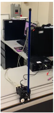
For our real-time experiments we use apparatus designed and provided by Quanser Consulting Inc. (119 Spy Court Markham, Ontario, L3R 5H6, Canada). This includes a single inverted pendulum mounted on an IP02 servo plant (pictured in Figure 3.11), a VoltPAQ amplifier, and a Q2-USB DAQ control board. The IP02 cart incorporates a Faulhaber Coreless DC Motor (2338S006) coupled with a Faulhaber Planetary Gearhead Series 23/1. The cart is also equipped with a US Digital S1 single-ended optical shaft encoder. The detailed technical specifications can be found in reference [63]. A diagram of our experimental setup is included in Figure 3.12.
3.4.2 Design Specifications
The goal of our real-time experiment is to stabilize the inverted pendulum in the upright position with minimal cart movement and control e↵ort. The weightsQ 0 andR >0 in the cost functional (3.4) must be chosen so that the system satisfies the following design performance requirements specified:
1. Regulate the pendulum angle around its upright position and never exceed a ± 1-degree-deflection from it, i.e. |↵|1.0 .
Figure 3.11: Single inverted pendulum mounted on a Quanser IP02 servo plant.
IP02
Amplifier
DAQ Computer
Control Signal
Pendulum Angle & Cart Position Pendulum Encoder
Cart Encoder
Amplifier Command Motor Connector
Figure 3.12: Diagram of experimental setup.
3.5
Experimental Results
Our Experimental results were obtained using Simulink in MATLAB and Quanser’s QuArc real-time control software. Our Simulink diagrams are provided in Appendix B.4.
3.5.1 Constant Weighting Matrices
The choice of the weighting matrices has a great e↵ect on the performance of the controller. In order to strongly penalize non-zero positions, the state weight Qmust be chosen with large weights on the positions and small weights on the velocities. The value of R needs to be suf-ficiently large to ensure that the power amplifier doesn’t go into saturation and to prevent excessive cart movement, however, if it is too large then the states might deviate from the zero position too much.
com-bination of values forQ andR, we use the following tuning procedure based on the procedure described by Quanser in [67]:
1. Perform a simulation with a particular choice for Qand R using the Simulink diagrams provided in B.3. Study the resulting state response and control e↵ort required. If the state response and control e↵ort are within the desired ranges then move onto the next step. Otherwise, adjust the values in Q and R, and run the simulation again. To adjust the values consider the following:
• If the cart’s position deviates too much from the center, then try increasing Q11 and/or decreasing Q22.
• If the pendulum’s angle deviates too much from the upright position, then try in-creasing Q22, and/or decreasing Q11.
• If the motor input voltage goes into saturation, try increasing R and/or decreasing Q11 together with Q22.
2. If the simulation results are satisfactory, then test the Q and R matrices in real-time using the Simulink diagrams provided in Appendix B.4. Adjust the values of Q and R until the state responses and the required control e↵ort are satisfactory. While adjusting the values, use the considerations from the previous step. If the cart is too “hyperactive” and vibrates excessively, then try increasingR and/or decreasingQ11 together withQ22.
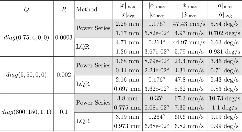
and 3.2 provide a summary of the analysis of the state responses and the control e↵ort for these three pairs of weighting matrices.
Table 3.1: Summary of stabilization state response with di↵erent weighting matrices.
Q R Method |x|max |↵|max |x˙|max |↵˙|max
|x|avg |↵|avg |x˙|avg |↵˙|avg
diag(0.75,4,0,0) 0.0003
2.25 mm 0.176 47.43 mm/s 5.84 deg/s Power Series
1.17 mm 5.82e-02 4.97 mm/s 0.702 deg/s
LQR 4.71 mm 0.264 44.97 mm/s 6.63 deg/s 1.26 mm 3.67e-02 5.79 mm/s 0.931 deg/s
diag(5,50,0,0) 0.002
1.68 mm 8.79e-02 24.4 mm/s 3.46 deg/s Power Series
0.44 mm 2.24e-02 4.31 mm/s 0.71 deg/s
LQR 2.16 mm 0.176 47.8 mm/s 5.43 deg/s
0.697 mm 3.62e-02 5.62 mm/s 0.83 deg/s
diag(800,150,1,1) 0.1
3.8 mm 0.35 67.3 mm/s 10.73 deg/s Power Series
0.775 mm 5.08e-02 7.35 mm/s 1.1 deg/s
LQR 3.19 mm 0.264 60.6 mm/s 9.19 deg/s
0.973 mm 6.68e-02 6.82 mm/s 0.99 deg/s
Table 3.2: Summary of control e↵ort with di↵erent weighting matrices.
Q R Method Vmax |Vm|avg R030|Vm|dt
Power Series 1.9 Volts 0.328 Volts 9.85 Volts diag(0.75,4,0,0) 0.0003
LQR 2.23 Volts 0.38 11.26
Power Series 1.77 Volts 0.32 Volts 9.57 Volts diag(5,50,0,0) 0.002
LQR 2.11 Volts 0.37 11.2
Power Series 2.9 Volts 0.41 Volts 12.33 Volts diag(800,150,1,1) 0.002
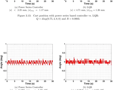
(a) Power Series Controller
|x| < 2.25 mm,|x|avg = 1.17 mm
(b) LQR
|x|<4.71 mm,|x|avg= 1.26 mm
Figure 3.13: Cart position with power series based controller vs. LQR:
Q=diag(0.75,4,0,0) andR= 0.0003.
(a) Power Series Controller
|↵| < 0.176 ,|↵|avg = 5.87e-02
(b) LQR
|↵|<0.264 ,|↵|avg= 3.67e-02
Figure 3.14: Pendulum’s angle with power series based controller vs. LQR:
(a) Power Series Controller
|x˙| < 47.43 mm/s,|x˙|avg = 4.97 mm/s
(b) LQR
|x˙|<44.97 mm/s,|x˙|avg= 5.79 mm/s
Figure 3.15: Cart velocity with power series based controller vs. LQR:
Q=diag(0.75,4,0,0) andR= 0.0003.
(a) Power Series Controller
|↵˙| < 5.84 deg/s,|↵˙|avg = 0.702 deg/s
(b) LQR
|↵˙|<6.63 deg/s,|↵˙|avg= 0.931 deg/s
Figure 3.16: Pendulum’s angular velocity with power series based controller vs. LQR:
(a) Power Series Controller
|Vm| < 1.R9 Volts,|Vm|avg = 0.328 Volts, 30
0 |Vm|dt = 9.85
(b) LQR
|Vm| < 2.R23 Volts,|Vm|avg = 0.376 Volts, 30
0 |Vm|dt = 11.26
Figure 3.17: Control e↵ort with power series based controller vs. LQR:
Q=diag(0.75,4,0,0) andR= 0.0003.
(a) Power Series Controller
|x| < 1.68 mm,|x|avg = 0.44 mm
(b) LQR
|x|<2.16 mm,|x|avg= 0.697 mm
Figure 3.18: Cart position with power series based controller vs. LQR:
(a) Power Series Controller
|↵| < 8.79e-02 ,|↵|avg = 2.24e-02
(b) LQR
|↵|<0.176 ,|↵|avg= 3.62e-02
Figure 3.19: Pendulum’s angle with power series based controller vs. LQR:
Q=diag(5,50,0,0) andR= 0.002.
(a) Power Series Controller
|x˙| < 24.4 mm/s,|x˙|avg = 4.31 mm/s
(b) LQR
|x˙|<47.8 mm/s,|x˙|avg= 5.62 mm/s
Figure 3.20: Cart velocity with power series based controller vs. LQR:
(a) Power Series Controller
|↵˙| < 3.46 deg/s,|↵˙|avg = 0.71 deg/s
(b) LQR
|↵˙|<5.43 deg/s,|↵˙|avg= 0.83 deg/s
Figure 3.21: Pendulum’s angular velocity with power series based controller vs. LQR:
Q=diag(5,50,0,0) andR= 0.002.
(a) Power Series Controller
|Vm| < 1.R77 Volts,|Vm|avg = 0.32 Volts
30
0 |Vm|dt = 9.57
(b) LQR
|Vm| < 2.R11 Volts,|Vm|avg = 0.37 Volts
30
0 |Vm|dt = 11.2
Figure 3.22: Control e↵ort with power series based controller vs. LQR:
(a) Power Series Controller
|x| < 3.8 mm,|x|avg = 0.775 mm
(b) LQR
|x|<3.19 mm,|x|avg= 0.973 mm
Figure 3.23: Cart position with power series based controller vs. LQR:
Q=diag(800,150,1,1) andR= 0.1.
(a) Power Series Controller
|↵| < 0.35 ,|↵|avg = 5.08e-02
(b) LQR
|↵|<0.264 ,↵avg= 6.68e-02
Figure 3.24: Pendulum’s angle with power series based controller vs. LQR:
(a) Power Series Controller
|x˙| < 67.3 mm/s,|x˙|avg = 7.35 mm/s
(b) LQR
|x˙|<60.6 mm/s,|x˙|avg= 6.82 mm/s
Figure 3.25: Cart velocity with power series based controller vs. LQR:
Q=diag(800,150,1,1) andR= 0.1.
(a) Power Series Controller
|↵˙| < 10.73 deg/s,|↵|avg = 1.1 deg/s
(b) LQR
|↵˙|<9.19 deg/s,|↵|avg= 0.99 deg/s
Figure 3.26: Pendulum’s angular velocity with power series based controller vs. LQR:
(a) Power Series Controller
|Vm| < 2R.9 Volts,|Vm|avg = 0.41 Volts, 30
0 |Vm|dt = 12.33
(b) LQR
|Vm| < 2.R59 Volts,|Vm|avg = 0.392 Volts, 30
0 |Vm|dt = 11.77
Figure 3.27: Control e↵ort with power series based controller vs. LQR:
Q=diag(800,150,1,1) andR= 0.1.
3.5.2 State-Dependent Weighting Matrix
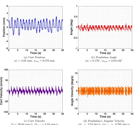
Table 3.3: Summary of stabilization state response and control e↵ort for the power series based controller with state-dependentQvs. controllers withQ=diag(800,150,1,1).
Method |x|max |↵|max |x˙|max |↵˙|max Vmax |Vm|avg R030|Vm|dt
|x|avg |↵|avg |x˙|avg |↵˙|avg 3.05 mm 0.176 28.64 mm/s 3.53 deg/s Power Series with
state-dependent Q 0.579 mm 2.67e-02 4.53 mm/s 0.765 deg/s 1.82 V 0.358 V 10.73 V 3.8 mm 0.35 67.3 mm/s 10.73 deg/s
Power Series with
constant Q 0.775 mm 5.08e-02 7.35 mm/s 1.1 deg/s 2.9 V 0.41 V 12.33 V
3.19 mm 0.264 60.6 mm/s 9.19 deg/s LQR
0.973 mm 6.68e-02 6.82 mm/s 0.99 deg/s 2.59 V 0.392 V 11.77 V
Figure 3.28: Control E↵ort with power series based controller:
Q(X) =diag(800 + 5x2,150 + 2↵2,1 + ˙x2,1 + ˙↵2) andR= 0.1
|Vm|<1.82 Volts, |Vm|avg= 0.358 Volts,R 30
(a) Cart Position
|x|<3.05 mm,xavg= 0.579 mm
(b) Pendulum Angle
|↵|<0.176 ,↵avg= 2.67e-02
(c) Cart Velocity
|x˙|<28.64 mm/s,|x˙|avg= 4.53 mm/s
(d) Pendulum’s Angular Velocity
|↵˙| < 3.53 deg/s,|↵|avg = 0.765 deg/s
Figure 3.29: State response with power series based controller:
3.5.3 Disturbance Rejection
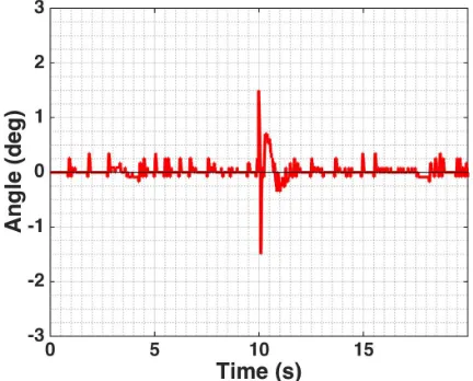
The performance of the power series based controller with both constant and state-dependent Qwas compared to the performance of the LQR controller in response to a 1.5 angular pulse disturbance. The three controllers performed very similarly, but the power series controller with state-dependentQrequired less voltage than the other two methods. Also notice, that for the power series method with state dependent Qthe maximum angular displacement was the same as the introduced disturbance, while the disturbance for the other two methods caused an overcompensated angular displacement in the opposite direction. The corresponding state responses and control e↵ort are provided in Figures 3.30-3.34. A summary of the analysis of the state responses and the control e↵ort in response to a 1.5 angular disturbance for the three methods is provided in Table 3.4.
Table 3.4: Summary of stabilization state response and control e↵ort with 1.5 pulse disturbance.
Method |x|max |↵|max |x˙|max |↵˙|max Vmax
Power Series with state-dependent Q 12.1 mm 1.5 183.7 mm/s 25.4 deg/s 7.65 Volts Power Series with constant Q 11.24 mm 1.76 197.4 mm/s 28 deg/s 8.81 Volts
(a) Power Series with Constant Q,|x|max= 11.24 mm (b) LQR,|x|max= 11.43 mm
(c) Power Series with State-Dependent Q,|x|max= 12.1 mm
(a) Power Series with Constant Q,|↵|max= 1.76 (b) LQR,|↵|max= 1.85
(c) Power Series with State-Dependent Q,|↵|max= 1.5
(a) Power Series with Constant Q,|x˙|max= 197.4 mm/s (b) LQR,|x˙|max= 181.3 mm/s
(c) Power Series with State-Dependent Q,
|x˙|max = 183.7 mm/s
(a) Power Series with Constant Q,|↵˙|max= 28 deg/s (b) LQR,|↵˙|max= 26.1 deg/s
(c) Power Series with State-Dependent Q,
|↵˙|max = 25.4 deg/s
(a) Power Series with Constant Q,|Vm|max= 8.81 Volts (b) LQR, |Vm|max= 8.82 Volts
(c) Power Series Controller,|Vm|max= 7.65 Volts
Chapter 4
Swing-up Control
4.1
Energy-based Controller
4.1.1 Pendulum’s Energy
One of the most popular control methods for swinging up the pendulum is where the control law is chosen such that the energy of the pendulum builds until reaching the upright equilibrium. This technique was first proposed and implemented by Astrom and Furuta [8, 9]. Here, we present a modified approach using a more complex dynamical model for the SIP system than the simplified model that is most commonly used. We also consider the electrodynamics of the DC motor that drives the cart, incorporate viscous damping friction as seen at the motor pinion, and account for the limitation of having a cart-pendulum system with a finite track length.
The total energy, Ep, of the pendulum at it’s hinge is given by the sum of it’s rotational
kinetic energy and it’s potential energy, so
Ep=
1 2Jp↵˙
2+M
p`pg(cos(↵) 1), (4.1)
whereJp, the pendulum’s moment of inertia at it’s hinge is defined as
Jp =
Z 2`p
0
r2Mp 2`p
dr= 4 3Mp`
2
p. (4.2)
Note that equation (4.1) di↵ers from the energy derived in Section 2.2.1 where we expressed the pendulum’s energy at it’s center of gravity and not at it’s hinge. Since our goal is to increase the energy of the pendulum until the upright position is reach, we must design a controller so that the condition
dEp