Real-Time Implementation of a Power Series
Based Nonlinear Controller for the Balance of a
Single Inverted Pendulum
Emese Kennedy, and Hien Tran,
Member, SIAM
Abstract—In this paper, we present the real-time implementa-tion of a nonlinear feedback controller for the balance of a single inverted pendulum based on the power series approximation to the solution of the Hamilton-Jacobi-Bellman (HJB) equation.
Index Terms—inverted pendulum, Hamilton-Jacobi-Bellman equation, nonlinear feedback control, real-time implementation, power series approximation.
I. INTRODUCTION
The single inverted pendulum (SIP) system is a classic example of a nonlinear system. It is considered as one of the most popular benchmarks of nonlinear control theory. Many nonlinear methods have been proposed for the swing-up and stabilization of a self-erecting inverted pendulum [1], however, most of these techniques are too complex and impractical for real-time implementation. In this paper, we present the successful real-time implementation of a nonlinear feedback control based on the power series ap-proximation to the solution of the Hamilton-Jacobi-Bellman equation [6], [7], [8], [9]. In our experiments, we have studied the disturbance rejection of our model and found that our controller is better than the traditional linear quadratic regulator. However, the analysis of our model’s disturbance rejection is beyond the scope of this paper and will be described in future publications.
II. SYSTEMDYNAMICS
A. Conventions
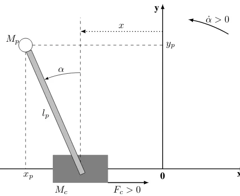
Figure 1 shows a diagram of the Single Inverted Pendulum (SIP) mounted on an IP02 linear cart. The positive sense of rotation is defined to be counterclockwise, when facing the cart. The perfectly vertical upward pointing position of the inverted pendulum corresponds to the zero angle, modulus 2π, (i.e.α= 0rad [2π]). The positive direction of the cart’s displacement is to the right when facing the cart, as indicated by the Cartesian frame of coordinates presented in Figure 1.
B. System Parameters
The model parameters and their values as specified by Quanser in [2] and [3] are provided in Table I.
Manuscript received October 30, 2014.
E. Kennedy is a graduate student in the Department of Mathematics, North Carolina State University, Raleigh, NC 27695 e-mail: [email protected]
H. Tran is with the Department of Mathematics, North Carolina State University, Raleigh, NC 27695 e-mail: [email protected]
0 x
y
Fc>0
Mc
x
yp
Mp
xp
lp
α
˙
[image:1.595.306.554.195.397.2]α >0
Fig. 1. Single inverted pendulum diagram.
TABLE I
INVERTEDPENDULUMMODELPARAMETERS
Symbol Description Value
Mw Cart Weight Mass 0.37 kg
M Cart Mass with Extra Weight 0.57 +Mwkg
Jm Rotor Moment of Inertia 3.90E-007 kg.m2
Kg Planetary Gearbox Gear Ratio 3.71
rmp Motor Pinion Radius 6.35E-003 m
Beq Equivalent Viscous Damping Coefficient 5.4 N.m.s/rad
Mp Pendulum Mass 0.230 kg
lp Pendulum Length from Pivot to COG 0.3302 m
Ip Pendulum Moment of Inertia about its COG 7.88E-003 kg.m2
Bp Viscous Damping Coefficient 0.0024 N.m.s/rad
g Gravitational Constant 9.81 m/s2
Kt Motor Torque Constant 0.00767 N.m/A
Km Back-ElectroMotive-Force Constant 0.00767 V.s/rad
Rm Motor Armature Resistance 2.6Ω
C. Equations of Motion
We use Lagrange’s method to derive the dynamic model of the system. In this approach, we consider the driving force, Fc, generated by the DC motor acting on the cart
through the motor pinion as the single input to the system. For Lagrange’s method we need to determine the Lagrangian of the system through the calculation of the system’s total potential and kinetic energies.
According to the reference frame definition presented in Figure 1, the coordinates of the pendulum’s center of gravity are characterized by:
To begin, we calculate the system’s total potential energy
VT. Since there is no elastic potential energy in the system,
the system’s potential energy is only due to gravity. The cart’s linear motion is horizontal with no vertical displacement. Therefore, the total potential energy is fully described by the pendulum’s gravitational potential energy,
VT =Mpglpcos(α(t)). (2)
Next, we will determine the system’s total kinetic energy
TT. The total kinetic energy is given by the sum of the
translational and rotational kinetic energies of both the cart and its mounted inverted pendulum. The cart’s translational kinetic energy,Tct, can be expressed as
Tct=
1 2M
d
dtx(t) 2
, (3)
while its rotational kinetic energy due to its DC motor,Tcr,
is given by
Tcr=
1 2
JmKg2 dtdx(t)
2
r2
mp
. (4)
Adding (3) and (4) we get that the cart’s total kinetic energy is
Tc =
1 2Mc
d
dtx(t) 2
where Mc=M+
JmKg2
r2
mp
. (5)
The mass of the pendulum is assumed to be concentrated at its Center Of Gravity (COG). Therefore, the pendulum’s transitional kinetic energy,Tpt, is given by
Tpt=
1 2Mp
d
dtxp(t) 2
+
d
dtyp(t) 2!
, (6)
where thex-coordinate of velocity of the pendulum’s center of gravity is
d
dtxp(t) = d
dtx(t)
−lpcos(α(t))
d
dtα(t)
(7)
and the y-coordinate is
d
dtyp(t) =−lpsin(α(t)) d
dtα(t)
. (8)
Furthermore, the pendulum’s rotational kinetic energy, Tpr
is given by
Tpr=
1 2Ip
d
dtα(t) 2
. (9)
Therefore, the total kinetic energy of the system is the sum of the four individual kinetic energies given by Equations (5)-(9). After rearranging and simplifying, the system’s total kinetic, TT, can be written as
TT =
1
2(Mc+Mp)
d
dtx(t) 2
−Mplpcos(α(t))
d
dtα(t) d dtx(t)
+1
2(Ip+Mpl
2
p)
d
dtα(t) 2
.
(10)
Note that the total kinetic energy can be expressed in terms of both the two generalized coordinates, x and α, and of their first derivatives.
Next, consider Lagrange’s equations for our system. By definition, the two Lagrange’s equations have the formal formulations
∂
∂t∂ dtdx(t)L
!
−
∂
∂xL
=Qx (11)
and
∂
∂t∂ dtdα(t)L
!
−
∂
∂αL
=Qα. (12)
In (11) and (12)Lrepresents the Lagrangian and is defined as the difference of the total kinetic energy and the total potential energy,
L=TT −VT. (13)
In (11),Qx is the generalized force applied on the
general-ized coordinatex, and is defined as
Qx(t) =Fc(t)−Beq
d dtx(t)
. (14)
Similarly, in (12),Qαis the generalized force applied on the
generalized coordinateα, which is defined as
Qα(t) =−Bp
d
dtα(t)
. (15)
It should be noted that in our current model the Coulomb friction applied to the cart, and the force on the cart due to the pendulum’s action have both been neglected.
Substituting into (11) and (12), and solving for the second-order time derivatives ofxandαresults in the two non-linear equations
d2
dt2x= −(Ip+Mpl 2
p)Beq
d
dtx
−(Mp2l3p+IpMplp) sin(α)
d
dtα 2
−Mplpcos(α)Bp
d
dtα
+ (Ip+Mpl2p)Fc
+Mp2l2pgcos(α) sin(α)
!
,
(Mc+Mp)Ip+McMpl2p+M
2
pl
2
psin
2(α)
(16)
and
d2
dt2α= (Mc+Mp)Mpglpsin(α)−(Mc+Mp)Bp
d
dtα
−Mp2lp2sin(α) cos(α)
d
dtα 2
−Mplpcos(α)Beq
d
dtx
+Mplpcos(α)Fc
!
,
(Mc+Mp)Ip+McMplp2+M
2
pl
2
psin
2(α) ,
(17)
force, Fc, to voltage input. Using Kirchoffs voltage law and
the physical properties of our system, we can easily show that
Fc=−
Kg2KtKm dtdx(t)
Rmr2mp
+KgKtVm
Rmrmp
. (18)
III. CONTROLLERDESIGN
A. Problem Statement
The state-space representation of our system has the form
d
dtX(t) =f(X(t)) +B(X(t))u(t) (19)
whereX, the system’s state vector is given by
XT(t) =
x(t), α(t), d dtx(t),
d dtα(t)
= [x1, x2, x3, x4],
(20) and the input u is set to equal the linear cart’s DC motor voltage, i.e. u = Vm. Based on equations (16)-(18) the
nonlinear function f(X)can be expressed as
f(X) =
0 0 1 0
0 0 0 1
0 0 a33 a34
0 0 a43 a44
x1
x2
x3
x4
+
0
0
M2
plp2gcos(x2) sin(x2)
D(X) (Mc+Mp)Mpglpsin(x2)
D(X)
(21) where
a33=
−(Ip+Mpl2p)(BeqRmr2mp+Kg2KtKm)
D(X)Rmrmp2
a34=−
(Mp2l3p+IpMplp) sin(x2)x4+Mplpcos(x2)Bp
D(X)
a43=−
(Mplpcos(x2))(BeqRmrmp2 +Kg2KtKm)
D(X)Rmr2mp
a44=−
(Mc+Mp)Bp+Mp2lp2sin(x2) cos(x2)x4
D(X)
and
D(X) = (Mc+Mp)Ip+McMpl2p+M
2
pl
2
psin
2
(x2).
Similarly, B(X(t))can be expressed as
B(X(t)) =
0
0
(Ip+Mpl2p)KgKt
D(X)Rmrmp
Mplpcos(x2)KgKt
D(X)Rmrmp
. (22)
Equation (22) can be linearized as
B=
0
0
(Ip+Mpl2p)KgKt ((Mc+Mp)Ip+McMpl2p)Rmrmp
Mplpcos(x2)KgKt ((Mc+Mp)Ip+McMpl2p)Rmrmp
.
ReplacingB(X(t))byB in (19) we obtain the nonlinear system
∂
∂tX(t) =f(X(t)) +Bu(X(t)) (23a)
X(0) =X0. (23b)
Now, consider the cost functional
J(X0, u) =
Z ∞
0
XTQX+Ru2dt, (24) whereQis a given constant-valued4×4symmetric positive-semidefinite matrix andRis a positive scalar. In the case of starting and balancing the inverted pendulum in the upright position, the optimal control problem is to find a state feedback control u∗(x) which minimizes the cost (24) for the initial conditionX0T = [0,0,0,0].
The function f is commonly linearized around the zero angle (i.e.α= 0) asf(X) =A0X. This linearization results
in the well-know linear quadratic regulator (LQR) problem, for which the optimal feedback control is given by
u∗(X) =−R−1BTP X,
where P is the unique symmetric positive-definite matrix solution to the algebraic Riccati equation
P A0+AT0P−P BR−
1BTP+Q= 0.
(25)
The theories for the LQR problem have been well-established, and multiple stable and robust algorithms for solving (25) have already been developed and are well documented in the literature and in textbooks [4], [5].
In our case, where f is nonlinear, the optimal feedback control is given by
u∗(X) =−1
2R
−1BTS X(X),
where the functionS is the solution to the Hamilton-Jacobi-Bellman (HJB) equation
SXT(X)f(X)−1
4S
T
X(X)BR−
1BTS
X(X) +XTQX= 0.
(26) It is well know that the HJB equation is very difficult to solve analytically. Several efforts have been made to numerically approximate the solution of the HJB equation in order to obtain a usable feedback control [6]. The following section describes one of these methods as it applies to the SIP system.
B. Power Series Approximation
The following method was adapted for the SIP system based on [6]. As it has been done by Garrard and others in references [7], [8], [9], the solution of the HJB equation can be numerically approximated using its power series expansion
S(X) =
∞
X
n=0
Sn(X),
where each Sn(X) = O(Xn+2). Similarly, the nonlinear
functionf(X)can be approximated by
f(X) =A0X+
∞
X
n=2
with fn(X) = O(Xn). In our implementation, the power
series of f was calculated using the MATLAB function
taylor from the Symbolic Math Toolbox. These expan-sions can be substituted into the HJB equation (26) to yield
"∞
X
n=0
(Sn)TX
# " A0X+
∞
X
n=2
fn(X)
#
−1
4
"∞ X
n=0
(Sn)TX
#
BR−1BT "∞
X
n=0
(Sn)X
#
+XTQX = 0.
We can separate out powers of X to obtain a series of equations,
(S0)TXA0X−
1 4(S0)
T XBR−
1BT(S
0)X+XTQX= 0, (27)
(S1)TXA0X−
1 4(S1)
T XBR−
1BT(S
0)X
−1
4(S0)
T XBR
−1BT(S
1)X+ (S0)TXf2(X) = 0,
(28)
(Sn)TXA0X−
1 4
n
X
k=0
(Sk)TXBR
−1BT(S n−k)X
+
n−1
X
k=0
(Sk)TXfn+1−k(X)
= 0,
(29)
wheren= 2,3,4, . . ..
The solution of equation (27) is
S0(X) =XTP X,
where P solves (25). As described earlier this gives the standard linear control. It is possible to solve equations (28)-(29) for Sn, n = 1,2,3, . . ., by making Sn a scalar
polynomial containing all possible combinations of products of the state elements with a total order of n+ 2. However, this method can get very complicated quickly. In [7], Garrard proposed a very easy method of finding(S1)X and obtaining
a quadratic type control.
Instead of the polynomial representation, we may use the solution of (27) and make the substitution(S0)X= 2P X in
equation (28) to obtain
(S1)TXA0X−
1 4(S1)
T XBR
−1BT(2P X)
−1
4(2X
T
P)BR−1BT(S1)X+ (2XTP)f2(X) = 0.
This can be rearranged to yield
XT
AT0(S1)X−P BR−1BT(S1)X+ 2P f2(x)= 0,
which is satisfied when
(S1)X =−2(AT0 −P BR
−1BT)−1P f 2(X).
This along with the (S0)X term give a quadratic feedback
control law of the form
u∗(X) =−R−1BT
P X−(AT0 −P BR−1BT)−1P f2(X).
(30) The series expansion off(X)in our case doesn’t contain any quadratic terms (i.e. f2(X) = 0), so (28) is trivially solved
byS1= 0. In this case, by [6], equation (29) forn= 2will
be of the form
(S2)TXA0X−
1 4(S2)
T XBR
−1BT(S
0)X
−1
4(S0)
T XBR−
1BT(S
[image:4.595.375.478.51.268.2]2)X+ (S0)TXf3(X) = 0
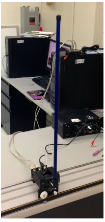
Fig. 2. Single inverted pendulum mounted on a Quanser IP02 servo plant.
IP02
Amplifier
DAQ
Computer
Control Signal
Pendulum Angle & Cart Position Cart Encoder
Pendulum Encoder
Amplifier Command Motor Connector
Fig. 3. Diagram of experimental setup.
which is exactly the same form as (28) except that S1 is
replaced beS2 andf2 is replaced by f3. Thus, the solution
is comparable to that of (28), with
(S2)X=−2(AT0 −P BR
−1BT)−1P f 3(X),
resulting in a feedback control of the form
u∗(X) =−R−1BTP X−(AT0 −P BR−1BT)−1P f3(X)
.
(31)
IV. REAL-TIMEIMPLEMENTATION
A. Apparatus
In our experiments we use apparatus designed and pro-vided by Quanser Consulting Inc (119 Spy Court Markham, Ontario, L3R 5H6, Canada). This includes a single inverted pendulum mounted on an IP02 servo plant (pictured in Figure 2), a VoltPAQ amplifier, and a Q2-USB DAQ control board. A diagram of our experimental setup is included in Figure 3.
B. Design Specifications
[image:4.595.306.525.293.409.2]Fig. 4. Main Simulink model diagram.
1) Regulate the pendulum angle around its upright posi-tion and never exceed a±1-degree-deflection from it, i.e.|α| ≤1.0◦.
2) Minimize the control effort produced, which is pro-portional to the motor input voltage Vm. The power
amplifier should not go into saturation in any case, i.e.
|Vm| ≤10V.
In order to strongly penalize non-zero positions, the state weight Q was chosen with large weights on the positions and no weights on the velocities. The particular choice of
Q = diag(5,50,0,0) and R = 0.002 were selected using the tuning procedure described by Quanser, however, within these considerations they are somewhat arbitrary.
C. MATLAB Implementation
Our control is implemented using Quanser’s QuArc real-time control software in MATLAB Simulink. The diagram of the main Simulink model is given in Figure 4. The controlu
is computed in real-time with a sampling rate of 1 kHz (1ms) using an Embedded Matlab Function block. The SIP+IP02 Actual Plant subsystem block that reads and computes the cart’s position and velocity, and the pendulum’s angle and angle velocity is taken from a model provided by Quanser.
D. Experimental Results
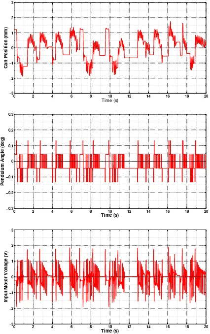
The experimental results are provided in Figure 5. As the graphs indicate, the results are well-within the desired model design specifications provided in Section IV-B. The pendulum’s angle is regulated around the upright position and never exceeds a±0.14◦-deflection from it. The amplifier input voltage always stays within ±1.91V and the power amplifier never goes into saturation. Furthermore, the cart’s movement is very minimal with no more than a 2 mm displacement in either direction.
V. CONCLUSION
We have described the successful real-time implementation of a new power series based nonlinear feedback control method for the balance of a single inverted pendulum. Our experimental results fall within the desired design specifi-cations, however, further fine tuning of the weights Q and
R may yield even better results with lower control effort and more accurate position tracking. Future work includes a more in-depth analysis of the system’s disturbance rejection as well as the implementation of another nonlinear controller based on the state-dependent Riccati equation.
0 2 4 6 8 10 12 14 16 18 20
−3 −2 −1 0 1 2 3
Time (s)
Cart Position (mm)
0 2 4 6 8 10 12 14 16 18 20
−0.3 −0.2 −0.1 0 0.1 0.2 0.3
Time (s)
Pendulum Angle (deg)
0 2 4 6 8 10 12 14 16 18 20
−3 −2 −1 0 1 2 3
Time (s)
Input Motor Voltage (V)
Fig. 5. Real-time experimental results. The top plot shows the actual (red) versus the desired (blue) cart position. The middle plot shows the angle of the pendulum, and the bottom plot shows the motor input voltage.
REFERENCES
[1] O. Boubaker, “The inverted pendulum benchmark in nonlinear control theory: A survey,”International Journal of Advanced Robotic Systems, vol. 10, pp. 1–9, 2013.
[2] IP01 and IP02 User Manual, Quanser Consulting, Inc.
[3] Single Inverted Pendulum (SIP) User Manual, Quanser Consulting, Inc. [4] H. T. Banks, R. C. Smith, and Y. Wang,Smart Material Structures: Modeling, Estimation, and Control. Chichester, England: Wiley, 1996. [5] I. Lasiecka and R. Triggiani,Differential and Algebraic Riccati Equa-tions with Application to Boundary/Point Control Problems. New York, NY: Springer Verlag, 1991.
[6] S. C. Beeler, H. T. Tran, and H. T. Banks, “Feedback control method-ologies for nonlinear systems,” Journal of Optimization Theory and Applications, vol. 107, no. 1, pp. 1–33, October 2000.
[7] W. L. Garrard, “Suboptimal feedback control for nonlinear systems,”
Automatica, vol. 8, pp. 219–221, 1972.
[8] W. L. Garrard and J. M. Jordan, “Design of nonlinear automatic flight control systems,”Automatica, vol. 13, pp. 497–505, 1977.
[image:5.595.322.535.59.398.2]