Deterministic Blind Subspace MIMO Equalization
Balaji Sampath
Electrical and Computer Engineering Department and Institute for Systems Research, University of Maryland, College Park, MD 20742, USA
Email: [email protected]
K. J. Ray Liu
Electrical and Computer Engineering Department and Institute for Systems Research, University of Maryland, College Park, MD 20742, USA
Email: [email protected]
Ye (Geoffrey) Li
School of Electrical and Computer Engineering, Georgia Institute of Technology, Atlanta, GA 30332, USA Email: [email protected]
Received 25 October 2001 and in revised form 14 February 2002
A subspace based approach for the blind multiple signal separation and recovery for MIMO systems is proposed in this paper. Instead of using the statistics of the received signal, the proposed algorithm exploits the received signal structure and the finite alphabet property of the desired signals. The finite alphabet property is used to remove the unknown unitary matrix that is associated with most of the statistics-based MIMO system identification algorithms. The proposed algorithm also incorporates an error-correcting procedure; therefore, it has more accuracy than the existing algorithms. Computer simulation results demonstrate that the algorithm can detect the signals and estimate channel parameters accurately with very few symbols, even under high noise and bad channel conditions.
Keywords and phrases:blind signal processing, subspace algorithm, MIMO system, equalization.
1. INTRODUCTION
Multiple transmit and receive antennas can be used in
wire-less communications to form input and
multiple-output (MIMO) systems to improve transmission capacity and performance. The first problem that we have to address before using MIMO communication systems is to identify and equalize MIMO systems, that is, to find system parame-ters, separate and recover signals. In this paper, we present blind subspace algorithm for MIMO system equalization. Since almost all MIMO systems can be modeled or approx-imated as FIR systems, we limit ourselves to linear FIR sys-tems.
A number of algorithms have been proposed for blind identification and equalization of channels with only one input. Traditionally, most blind equalization algorithms for
single-input and single-output (SISO) systems have been based on higher-order statistics [1, 2, 3, 4]. In the last few years, a number of second-order statistics based algo-rithms have been proposed in [5, 6, 7] to exploit the
cyclo-stationarity of oversampledcontinuousSISO communication
systems. Since an oversampled continuous SISO system is
equivalent to a discrete single-input and multiple-output
(SIMO) system, these algorithms can be regarded as address-ing the SIMO system identification problem as well. Recently, a number of subspace-based algorithms have been proposed in [8, 9, 10, 11, 12] for blind system identification. In partic-ular, we have proposed a new deterministic subspace-based algorithm in [11, 12] which addresses blind equalization of oversampled continuous SISO (or equivalently discrete SIMO) systems. Compared with other algorithms in the liter-ature, this algorithm has much better performance. However, it requires that the number of outputs equal to the FIR chan-nel length, which is very restrictive in reality. In Section 2, we generalize this algorithm, remove this restriction, and
study the performance of the algorithm under different
over-sampling rates. The approach used to generalize the SIMO identification algorithms can be also used to generalize the MIMO identification algorithm developed in Section 3.
s(n)
h1(n)
h2(n)
hK(n)
x1(n)
x2(n)
xK(n) .
.
. ...
(a)
s1(n)
sd(n)
h1,1(n)
h1,d(n)
hK,1(n)
hK,d(n)
x1(n)
xK(n) .
. .
. . .
. . .
. . .
. . .
(b)
Figure1: (a) SIMO System, (b) MIMO System.
MIMO problem is much more difficult to deal with. For
ex-ample, it can be shown that by using only the structure and no other extra information (like quantized inputs or knowl-edge of the statistics), we can only identify the system up to a unitary matrix. Nevertheless, a few algorithms that equal-ize MIMO systems have been discovered [10, 13, 14]. In particular, [10, 14] are subspace-based methods which use the ILSP method described in [15] and are iterative. The statistics-based algorithm in [13], like other statistics-based algorithms, needs a very long observation interval to equalize the system and is therefore not suited to fast changing envi-ronments, such as wireless communications. It is becoming greater to find MIMO system blind equalization algorithms that use smaller observation intervals, work well at high noise conditions, and give more accurate estimates. In Section 3, we develop an algorithm for MIMO systems that requires a
small observation interval. The effectiveness of the proposed
algorithms is demonstrated through computer simulation in Section 4.
2. GENERALIZED SUBSPACE ALGORITHM
FOR SIMO SYSTEMS
In [11, 12], we presented an algorithm for blind identifica-tion of oversampled continuous SISO systems under certain conditions. However, that algorithm requires that the over-sampling rate should be exactly the same as the length of the FIR channel. Although in most cases this constraint will not create any problems. In some cases, too high oversampling rates will cause the impulse response matrix to become very ill-conditioned, which leads to poor channel estimates. Af-ter describing the mathematical model of SIMO systems, we will present a generalized subspace algorithm that does not require the constraint.
2.1. Problem statement
The mathematical model of 1-input and K-output systems
can be illustrated as in Figure 1a. The sequence s(n) is sent
throughKlinear channelshi(n),i=1, . . . , K. In the noiseless
case, the channel outputsxi(n), 1≤i≤K, can be expressed
as
xi(n)= J−1
j=0s
(n−j)hi(j), (1)
whereJ is the maximum length ofhi(·)’s. The problem we
propose to tackle here is the blind identification and equal-ization of SIMO systems, that is, to find an algorithm to es-timate the sequence s(n) given only the outputsxi(n). The
solution we presented in [11, 12] assumed thatK =J. Here
we will derive a more general algorithm without using the assumption.
For a givenn, define for 1≤i≤K,
xi(p)=
xi(p) xi(p+ 1) · · · xi(p+n−1)
T ,
s(p)=s(p) s(p+ 1) · · · s(p+n−1)T,
hi=
hi(0) hi(1) · · · hi(J−1)
T .
(2)
With the above definitions, equation (1) can be expressed as,
xi(p)=s(p) s(p−1) · · · s(p−J+ 1)hi, (3)
or
x1(p) x2(p) · · · xK(p)
=s(p) s(p−1) · · · s(p−J+ 1)H, (4)
whereHis aJ×Kmatrix defined as
H=h1 h2 · · · hK
. (5)
When developing the subspace algorithms in [11, 12], we
have assumed that the matrixHis square (i.e.,J = K) and
Unfortunately,Hneed not be a square matrix (and hence will not be invertible). Therefore, we are going to introduce a generalized algorithm to deal with the situation.
2.2. Generalized subspace algorithm
The algorithm developed in [11, 12] requires that H be a
square matrix. WhenHis not square, the generalized
algo-rithm is to modify this matrix to get a square, invertible ma-trix, without substantially changing (4). Without loss of
gen-erality, we assumeK≤J.
LetOj×kbe a j×kmatrix of zeros. DefineHˆ1 =Hand
ˆ
Hj+1recursively as,
ˆ
Now, define the following:
X(p)=x1(p) x2(p) · · · xK(p),
With the above definitions, we have the following equation:
X(p)=S(p)Hˆ. (8)
Now define the matrixΦas
Φ=
senting a matrix of zeros.
We can show thatΦcan be factored as
Φ=ΨH˜, (10)
From [11, 12, Lemma 3.2], we know that the probability that
Ψhas a one-dimensional null-space tends to 1 exponentially
with increasing n. We also know that the one-dimensional
null space is given byᏺ(Ψ),
So for all practical purposes we can assume thatΨhas a
one-dimensional null space. If we further assume thatHˆ is
invert-ible, it is easily seen thatΦhas a one-dimensional null-space
and that the null space ofΦis given by
ᏺ(Φ)=
Note thatΦis a matrix whose elements are the actual
chan-nel output samples—so we can apply some of the standard algorithms to find its null space—let the null space be
ᏺ(Φ)=cλ1 λ2 · · · λJ+j−1T:c∈
the channel response matrix, up to a multiplication factor. Thus, in the noiseless case we have identified the channel exactly.
The same algorithm can be used for noisy case. Instead
of finding a null vector of Φ, we find the smallest
singu-lar vector of Φ. To obtain a better estimate of the channel,
algorithm discussed in [11, 12]. Here we have a choice of several sampling rates (or equivalently several channels)
un-like [11, 12] where the sampling rate was fixed at J—by
choosing an appropriate sampling rate, it may be possible to overcome the problem of ill-conditionedness that is al-ways faced in blind equalization algorithms. In [11, 12], the ill-conditionedness problem was overcome by
choos-ing the effective channel length to be smaller thanJ. Here
the ill-conditionedness can be overcome by reducing the sampling rate itself. In Section 4, we present some simula-tion results comparing the performance of this algorithm
at different sampling rates. From the simulations we can
see that at least for very ill-conditioned matrices, the per-formance becomes better as the rate of over-sampling
de-creases. The reason for this counter-intuitive result1is that,
in very ill-conditioned matrices, increasing the sampling rate does not really increase the information content in the samples.
3. THE SUBSPACE ALGORITHM FOR THE MIMO SYSTEMS
In Section 2, we looked at the SIMO channel equalization problem. In this section, we tackle the MIMO channel case.
The mathematical model ofd-input/K-output MIMO
sys-tems can be illustrated as in Figure 1b. The d sequences
s1(n), . . . , sd(n) are sent through linear channels hi j(n) for
present below assumes thatK =Jd. By using the approach
that was presented in Section 2 for the SIMO case, this
algo-rithm can also be extended toK=Jdcase.
3.1. The MIMO subspace approach
First we define some matrices and derive some basic relations between them, and then prove Theorem 1. Based on these relations and Theorem 1, we then derive the MIMO subspace algorithm.
1Intuitively, higher sampling rate implies more information, which in general should lead to better performance.
H=
We then have the following equation:
X(p)=S(p)H. (19)
Now construct the matrixΦas
Φ=
with the number of block-rows beingJ, 0 representing a
ma-trix of zeros. Using (18) and (19), it is easy to see that the following identity holds:
Φ=ΨH˜, (21)
Below we prove thatΨhas ad-dimensional null space.
Theorem 1. If the vectorssi(j)for1≤i≤dand(p−J+ 1)≤ j≤(p+1)are independent, thenΨhas thed-dimensional null space given by
ᏺ(Ψ)=
Lemma 1. If theJ+ 1vectorsᏮ0,Ꮾ1, . . . ,ᏮJ are linearly in-dependent, then×nmatrix,Γ, with zero elements everywhere except the following elements:
Γii=Ꮾ1Ꮾ2· · ·ᏮJ,
Γi,i+1=Ꮾ0Ꮾ1· · ·ᏮJ−1
(24)
has a one-dimensional null space and
ᏺ(Γ)=ce1 e2 e3 · · · eJ
T
:c∈ . (25)
With the above lemma, we can now prove the theorem.
Proof of Theorem 1. Let On×k be an n×k matrix of zeros, Therefore,βiis given by
βi=
It can be seen that the following relation holds:
Ψiβi=0 for 1≤i≤d. (30)
Using Lemma 1 it can be seen that (30) implies that
βi=ci
Assuming further thatH is invertible, we can conclude
thatΦalso has ad-dimensional null space if the vectorssi(j),
for 1 ≤i ≤d, (p−J+ 1) ≤ j ≤(p+ 1), are independent.
But it is easy to see that asnincreases, the probability that
these vectors are not independent goes to zero exponentially
[11, 12]. Therefore, we conclude that asnincreases, the
prob-ability thatΦhas ad-dimensional null space increases
expo-nentially to 1.
Also from the expression for the null space of Ψ in
Theorem 1, it follows that the null space of Φcan be
writ-ten as
where the basis vectorsbiare
bi=
quired information aboutHas well as about the transmitted
sequences, for
Λ=Λe1 Λe2 Λe3 · · · ΛedJ, (34)
S(p)=X(p)Λ. (35)
Another important observation is that just the
knowl-edge of bi is enough to determine the ith transmitted
se-quence. The reason is that the J columns (from columns
(i−1)J + 1 to iJ) of Λ are from bi and the information
about theith transmitted sequence can be obtained by
post-multiplyingX(p) by theseJcolumns ofΛ.
3.2. The problem caused by thed-dimensionality of the null space
From the above relations, it is clear that if we have the ba-sis vectors, then we have solved the MIMO problem. Un-fortunately, the basis vectors are unknown. In the SIMO case, this problem does not arise since the null space is
one-dimensional. Here the null-space isd-dimensional and
stan-dard algorithms (like the SVD algorithm) can give us the null
space, but not the basis vectors that we need. Just arbitraryd
basis vectors for the null-space will not be enough—the basis vectors we need are special as given by (33). If we just choose a basis for the null space, what we end up with is a linear combination of the basis vectors, that is, vectors of the form
d
i=1kibi, whereki∈ . The problem that we therefore have
to address can be stated as follows:given the null space (and
some basis for it), find thedbasis vectors{bi}.
To solve this problem, we now make use of the discrete nature of the transmitted sequence. In what follows, for the
sake of simplicity in presentation, we focus only on thed=2
case. The points discussed below can be easily generalized to arbitraryd.
Our two basis vectorsb1andb2lie in the null space. So if we have any other two independent vectors which belong to the null space, then our basis vectors are just linear combina-tions of those two vectors. We write this mathematically. Let
γ1andγ2be any two vectors in the null space obtained from
Φ, then
b1=xγ1+yγ2, b2=zγ1+wγ2, (36)
for somex, y, z, w∈ . The problem now reduces to finding
Table1: Procedure for findingxandy.
Step 1.Choose two independent vectors,γ1andγ2, in the null space.
Step 2.Choose somexandy.
Step 3.Substitute these values ofx,y,γ1, andγ2in (36). This gives us an estimate ofb1.
Step 4.Using this estimatedb1and (35) obtain an estimate for the transmitted sequence.
We had previously made the observation that just the
knowledge ofb1 is enough to determine the first sequence.
This now boils down to the statement that just the knowledge
ofxandy, the weighting factors ofγ1andγ2, is enough to
determine the first sequence. We will make use of this
obser-vation below to solve forxandyand hence the transmitted
sequence. Table 1 describes the procedure to findxandy.
The big question is of course: what if the estimate ofx
and yis wrong? What criterion should be used to find out
whether our estimate forxandyis correct? One reasonable
criterion is the following:whenever the transmitted sequence
obtained fromxand yis a proper transmitted sequence, then we can assume that the estimate ofxandyis correct. Note that we do not know the exact transmitted sequence but we do know the symbol constellation of the transmitted sequence.
So we can define aproper transmitted sequenceto be any
se-quence with elements from the signal constellation.
Using the idea presented above to check whether any
as-sumedxandyis correct, we have Table 2 for estimating the
transmitted sequence (and the channel responses). Here are some comments on Table 2.
(1) To find x and y in Step 3 in the algorithm,
two-dimensional search over real numbers is required. Theproper
transmitted sequencecriterion defines the correct estimate by
the fact that at the correct estimates ofxandy, all the
ele-ments of the estimated transmitted sequence will lie in the signal constellation. In a noisy situation, instead of the
cor-rect estimates ofxandy, we will have the optimum estimates
of x and yand the condition that the estimated
transmit-ted sequence should lie in the signal constellation will be
re-placed by the following:denote the estimated transmitted
se-quence to bev. Find the constellation-sequenceuclosest2tov,
that is, to findxandythat minimize u−v .
(2) If signal constellation is the same for both the
se-quences, there will be two sets ofxand yat which the
es-timated transmitted sequence will lie in (or in the noisy case be very close to a sequence with elements in) the signal con-stellation. These represent the two transmitted sequences and with one search we can find both the transmitted sequences. (3) As we can see in Section 3.3, the two-dimensional search can actually be reduced to a one-dimensional search.
2We can choose any sensible criterion for closeness—for most practi-cal cases, we can either use the nearest neighbor rule or more simply just perform an element by element quantization. In our simulations we have adopted the later approach of element by element quantization.
Table2: MIMO-subspace algorithm (without error correction).
Step 1.Construct the matrixΦ.
Step 2.Find any two linearly independent vectors,γ1and γ2, in the null space ofΦ.
Step 3. Using the procedure described above and using theproper transmitted sequencecriterion for correctness, search for the correctxandyover all possible values they can take.
3.3. Complexity reduction
To reduce the computational complexity, it would be better if we could manage with just a one-dimensional search instead of a two-dimensional search over reals. It is in fact possible to reduce the two-dimensional search to a one-dimensional search. Furthermore, it does not involve any loss in accuracy of estimate.
There are many ways in which this can be done. For
ex-ample, we can just setx = 1 and search over all values ofy
from−∞to∞. We can normalize each vector obtained and
this gives all possible3normalized vectors in the null space.
But we end up with problems if for exampleb1=γ2, for then
ywill have to be∞which is not practically reachable through
any search algorithm. So from a practical point of view this
approach and other similar approaches are not very effective.
We found the following procedure most advantageous from a computational angle.
(1) Perform Gram-Schmidt orthonormalization
proce-dure on the two vectors,γ1 andγ2 and obtain the two
or-thonormal vectorsδ1andδ2. Letτ1andτ2be the first 2J ele-ments ofδ1andδ2, respectively.
(2) Minimize the following over 0≤θ≤2π,
a−quant(a), (37)
whereais the estimate of the transmitted sequence given by
a=X(p+ 1)cos(θ)τ1+ sin(θ)τ2
(38)
and quant(x) is the element by element quantization of x,
where the quantization maps each element ofxto its nearest
point in the signal constellation. Figure 2 shows a sample plot
of a−quant(a) versusθ(in the noisy case).
The actual estimates of the two transmitted sequences are the quantized versions of the estimated sequences obtained
from the two values ofθat the two minima.
3.4. Error-correcting least squares MIMO algorithm We have so far made substantial use of the structure inher-ent in the output samples. Although we have also used the fact that the transmitted sequence is quantized, we have not
−2 −1.5 −1 −0.5 0 0.5 1 1.5 2 Angle in radians
0 0.1 0.2 0.3 0.4 0.5 0.6 0.7 0.8
Quantizatio
n
er
ro
r
Figure2: One sample plot of a−quant(a) versusθ.
exploited it fully. The ECLS algorithm discussed in [11, 12] does this very effectively and we can apply it here as well.
The crucial point in the ECLS algorithm is the observa-tion that in almost all practical cases, if the initial estimate is close enough to the desired optimum, then we can reach the optimum by searching over a smaller area around initial es-timate. The great reduction in the computational complexity
comes from the fact thatnsmall searches is just linear
com-plexity whereas one search over the whole area4will have a
complexity ofnp, wherepis the dimension in which we are
searching.
By applying this same idea here, we can reduce the search complexity greatly. The only problem is that we have two es-timated sequences rather than one. So there are many ways in which we can do a smaller search. We can at each stage search over all possible one-element deviations for each transmitted sequence and then choose those one-element deviations for each sequence which corresponds to the overall optimum. The algorithm which does this is shown in Table 3.
But since we are only dealing with finite sequences, there is an even more simpler way of using error-correction. Con-catenate the two sequences and apply the error correcting procedure on the combined 1D sequence. This is clearly only a subset of the previously described algorithm and so the performance of this will be degraded compared to the pre-vious. But the importance of this approach lies in the fact that it reduces the complexity substantially. In the case that the two transmitted sequences are independent, the assump-tion that we can search over the two sequences independently (which is what we are doing here) instead of a joint search for the best sequence-pair, is quite reasonable. Because of these advantages, in our simulations we use this approach. Although the ECLS-MIMO algorithm improves the perfor-mance in all cases, the improvement is especially important
4The word area has been used as a general term for the region of search, not to denote the two-dimensionality of the search region.
Table3: ECLS-MIMO algorithm.
Step 1.First let the search area be all the sequence-pairs which differ from thecurrent sequence-pairin at most one position for each sequence in the pair.
Step 2.Find thebestsequence-pair in this area. The best sequence-pair is the one which has the smallest least-squares error, that is, minimizes S(p)Hˆ −X(p) over all possibleHmatrices, where ˆS(p) is theS(p)-matrix that would be used in (21) if the actual transmitted sequences were the sequence-pairs in question.
Step 3.If this sequence is the same as thecurrent sequence-pairthen stop and decide that this is thebestestimate. Step 4. If this sequence is not the same as thecurrent sequence-pair then replace the current sequence-pair by this sequence-pair and start all over again from Step 1.
when the matrix H is ill-conditioned because the channel
and sequence estimates are not very accurate.
4. SIMULATION RESULTS
In this section, we present some simulation results for the two algorithms presented in this paper—the generalized SIMO and MIMO-subspace algorithms—and compare it with other algorithms, under the same channel and noise conditions.
4.1. Simulations results for the generalized SIMO algorithm
First, we present the results for the generalized SIMO-subspace algorithm and compare it with the results in [8, 9, 10]. Here we do not present the results for [11, 12] since the algorithm in [11, 12] assumes that the “numerical” chan-nel length is smaller than the actual chanchan-nel length and uses the shorter channel length for its computation which leads to its better performance. This approach to overcome the ill-conditionedness of the channel is complimentary to the lower sampling rate approach we have proposed in this pa-per and both the approaches can be used simultaneously to even further improve the performance.
For these simulations, we used a channel withJ = 4.
Oversampling it at four times the baud rate, the channel
ma-trixHwhich we used is given by
H=
0.04142 0.0216 −0.01959 −0.06035
−0.07025 −0.0241 0.08427 0.2351
0.3874 0.4931 0.5167 0.4494
0.3132 0.152 0.01383 −0.06754
. (39)
To quantify the ill-conditionedness or
well-conditioned-ness of a matrix we will use RCOND(X). RCOND(X) is an
estimate for the reciprocal of the condition of X in the
1-norm. If X is well conditioned, RCOND(X) is near 1.0. If X
is badly conditioned, RCOND(X) is near 0.0. For the
1 2 3 4 5 6 7 8
Figure3: Generalized subspace algorithm, (a), (b) 2-oversampling, (c), (d) 3-oversampling, and (e), (f) 4-oversampling. SNR=25 dB. (a),
0 2 4 6 8
n −0.2
0 0.2 0.4 0.6 0.8
h
[
n
]
(a)
0 2 4 6 8
n −0.2
0 0.2 0.4 0.6 0.8
h
[
n
]
(b)
0 2 4 6 8
n −0.5
0 0.5 1
h
[
n
]
(c)
0 2 4 6 8
n −0.5
0 0.5 1
h
[
n
]
(d)
Figure5: 20 estimates of the channel for (a) SNR=20 dB, (b) SNR=15 dB, (c) SNR=10 dB, and (d) SNR=5 dB for the oversampling
twice-subspace algorithm. 40 symbols.
very ill-conditioned matrix. If we oversample the channel at only twice the baud rate (as opposed to the four times over-sampling done above) and create a square matrix using the method presented in Section 2, the RCOND of the matrix thus obtained is 0.0123. This is still an ill-conditioned ma-trix but the condition number is five times better. By choos-ing the samplchoos-ing instants appropriately we can even make
the RCOND =0.0186—but since we have no hold over the
sampling instants, for our simulations we assume a sampling such that we get a lower condition number. Similarly, de-pending on the sampling instants, sampling at three times the baud rate can give us square matrices with RCOND num-bers 0.0021, 0.0046, or 0.0134. For our simulations we have assumed the sampling rates to be such that the RCOND
number is the worst of the possible values, that is, RCOND=
0.0021. Since the matrices are so ill-conditioned, it is neces-sary to use error-correction and all results presented below are with error correction.
To obtain a performance measure of the channel estima-tion, the normalized root-mean-square error (NRMSE) of the estimator is defined by
NRMSE= 1
h
1
M M
i=1
hˆ
(i)−h2, (40)
whereMis the number for independent trials, and ˆh(i)is the
estimate of the channel from theith trial. Figure 6a shows
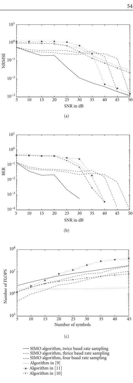
the NRMSE versus SNR for different algorithms. In Figure 6b
we have shown the bit error rate (BER) in estimating the
transmitted sequences for the different algorithms. Figure 6c
shows the computational complexity of different algorithms
(measured by the number of floating point operations— FLOPS in MATLAB). As we can see from these figures, the BER is quite small and drops very sharply for all the sub-space algorithm with an increase in the SNR. Also we can clearly see that the values of both the NRMSE and the BER for the generalized subspace algorithms presented here are lower than for other algorithms in the literature in the low SNR situation. In particular, the twice baud rate sampling case consistently outperforms the rest.
channel estimates using the 2-times oversampling subspace algorithm with only 40 symbols for 20, 15, 10, and 5 dB SNR, respectively.
The figures clearly demonstrate how as the condition number of the matrix becomes better (with lower sampling the condition number can get better), the performance im-proves. Sampling at twice the baud rate improves the con-dition number and hence the performance as compared to sampling at 4 times the baud rate. Also, just reducing the sampling rate also improves the performance—even though we chose the worst cases of sampling at thrice baud rate, still the performance is better than the 4-times baud rate sam-pling case.
Figure 6c is the computational complexity plot. It shows that the complexity of the generalized subspace algorithm presented here is comparable to those of the other algorithms in the literature. As should be expected, lowering the sam-pling increases the complexity—the reason being that the
lower the sampling rate, the bigger the effectiveH(with
zero-paddings) becomes. Since the complexity of the subspace approach (because of the singular value decomposition for finding the null space) depends on the size of this matrix, as this size increases, we can expect the complexity to also in-crease.
4.2. Simulations results for the MIMO algorithm
We will now present the results for the MIMO-subspace algo-rithm and compare it with the MIMO equalization algoalgo-rithm presented in [14]. We will present the results first without using error-correction and then with error-correction and
demonstrate the algorithm’s effectiveness in both cases.
The simulation study presented here is for the case when
d =2,K =4, andJ =2. The impulse responses used in the
simulation for both the algorithms is given as
H=
0.1667 0.1057 −0.0665 0.3232
0.4813 0.5333 0.4369 0.3846
0.2804 −0.0505 0.2208 −0.0067
0.3730 0.4744 0.4296 0.5090
. (41)
Figures 7a and 7b show the estimates5of the channel
re-sponse using the algorithm in [14] for SNR=25 dB. In both
cases, the length of the observation interval covers 100 sym-bols. Figures 7c and 7d show the estimates obtained by using the subspace algorithm without error correction and using an observation interval of only 50 symbols. The SNR in this case is also 25 dB. These figures show that the subspace algo-rithm (even without error correction) performs much better than the algorithm in [14].
Figures 8a and 8b show the NRMSE of the algorithm versus SNR for the two input sequences. In Figures 9a and 9b we have shown the BER in estimating the two input se-quences. As can be seen from the figure, the BER drops very
5We have combined the channel responses of the four channelsh i,1(n), 1≤i≤4, and the four channelshi,2(n), 1≤i≤4, to form the two channel responses shown in the figures.
5 10 15 20 25 30 35 40 45 50
SNR in dB 10−3
10−2 10−1 100 101
NRMSE
(a)
5 10 15 20 25 30 35 40 45 50
SNR in dB 10−4
10−3 10−2 10−1 100 101
BER
(b)
5 10 15 20 25 30 35 40 45
Number of symbols 105
106 107 108
Nu
m
b
er
o
f
F
L
O
P
S
(c)
____ ____
...
...
SIMO algorithm, twice baud rate sampling SIMO algorithm, thrice baud rate sampling SIMO algorithm, four baud rate sampling Algorithm in [9]
Algorithm in [11] Algorithm in [10]
Figure6: (a) NRMSE versus SNR, 35 symbols. (b) BER versus SNR,
1 2 3 4 5 6 7 8
n −0.8
−0.6
−0.4
−0.2 0 0.2 0.4 0.6 0.8
h
[
n
]
(a)
1 2 3 4 5 6 7 8
n −0.1
0 0.1 0.2 0.3 0.4 0.5 0.6
h
[
n
]
(c)
1 2 3 4 5 6 7 8
n −0.6
−0.4
−0.2 0 0.2 0.4 0.6 0.8
h
[
n
]
(b)
1 2 3 4 5 6 7 8
n −0.1
0 0.1 0.2 0.3 0.4 0.5 0.6
h
[
n
]
(d)
Figure7: (a), (b) Algorithm in [14], 100 symbols, SNR=25 dB. (c), (d) MIMO subspace algorithm without error correction, 50 symbols,
SNR=25 dB.
____
_ _ _
...
____
_ _ _
...
10 15 20 25 30 35 40 45 50
SNR (dB) 10−3
10−2 10−1 100
NRMSE
Subspace algorithm (with error correction) Subspace algorithm (without error correction) Algorithm in [13]
10 15 20 25 30 35 40 45 50
SNR (dB) 10−3
10−2 10−1 100
NRMSE
Subspace algorithm (with error correction) Subspace algorithm (without error correction) Algorithm in [13]
____
_ _ _
...
____
_ _ _
...
10 15 20 25 30 35 40 45 50
SNR (dB) 10−4
10−3 10−2 10−1 100
BER
Subspace algorithm (with error correction) Subspace algorithm (without error correction) Algorithm in [13]
10 15 20 25 30 35 40 45 50
SNR (dB) 10−4
10−3 10−2 10−1 100
BER
Subspace algorithm (with error correction) Subspace algorithm (without error correction) Algorithm in [13]
Figure9: BER versus SNR for the two input sequences. 100 symbols used for each estimate.
____ _ _ _
30 40 50 60 70 80 90 100
Number of symbols 106
107 108
Nu
m
b
er
o
f
F
L
O
P
S
Subspace algorithm (with error correction) Algorithm in [13]
Figure10: Computational complexity versus observation interval.
SNR=25 dB.
sharply for the proposed subspace algorithm (for both— with and without error correction) with an increase in the SNR. Also we can clearly see that both the values of the NRMSE and BER for the subspace algorithm are much lower than their values for the algorithm in [14]. Figure 10 shows the computational complexity of this algorithm (using er-ror correction) and the algorithm in [14]. As the number of symbols increases, the complexity of the algorithm in [14] rapidly increases and becomes much more computation-ally intensive than the MIMO subspace algorithm presented here.
5. CONCLUSIONS
In this paper, we generalized the basic subspace algorithm presented in [11, 12]. This generalization allows us to use it even in cases when the sampling rate cannot be chosen to be equal to the FIR channel length. We compared this result to other algorithms and found that this algorithm is more gen-eral than the one in [11, 12] and performs much better than other algorithms in the literature [8, 9, 10]. The simulation study also showed that for ill-conditioned channels as the sampling rate is reduced, the performance becomes better.
In this paper, we have also proposed a new algorithm for the blind equalization and identification of MIMO systems. This algorithm uses a subspace based approach in combina-tion with a searching procedure based on the finite alpha-bet property of the input sequence. As the simulation results show, this algorithm needs fewer symbols than the algorithm in [14] for obtaining a good estimate of the MIMO channel response as well as the transmitted sequences. The accuracy of the channel estimate is also better than [14]. Finally, this algorithm is quite robust to noise and computationally also
more efficient than the algorithm in [14].
APPENDIX
Proof of Lemma 1. Let the vector β be a vector in the null
space ofΓwhere
β=β1,1, β2,1, . . . , βJ,1, β1,2, β2,2, . . . ,
βJ,2, . . . ,β1,J, β2,J, . . . , βJ,J
T .
(A.1)
Then
From this equation, and, using the fact that since the vectors
Ꮾ0,Ꮾ1, . . . ,ᏮJ are linearly independent, a linear
combina-tion of them cannot be zero unless all the corresponding
co-efficients are zero, we get the following equations:
β1,i=0 ∀i=2,3, . . . , J−1, J,
β1,i−β2,i+1=0 ∀i=1,2,3, . . . , J−1,
β2,i−β3,i+1=0 ∀i=1,2,3, . . . , J−1,
.. .
βJ−1,i−βJ,i+1=0 ∀i=1,2,3, . . . , J−1,
βJ,i=0 ∀i=1,2,3, . . . , J−1.
(A.3)
From these equations it can be concluded that βi, j fori =
j are all zero andβ1,1 = β2,2 = · · · = βJ,J. This means that
the vectorβis fixed up to a multiplication factor and since
βis an arbitrary vector in the null space ofΓ, we infer that
Γhas a one-dimensional null space generated by the vector
[e1 e2 e3 · · · eJ]T.
REFERENCES
[1] G. Giannakis, Y. Inouye, and J. Mendel, “Cumulant-based identification of multichannel moving average models,”IEEE Trans. on Automatic Control, vol. 34, no. 7, pp. 783–787, 1989. [2] G. Giannakis and J. Mendel, “Identification of non-minimum phase systems using higher-order statistics,” IEEE Trans. Acoustics, Speech, and Signal Processing, vol. 37, no. 3, pp. 360–377, 1989.
[3] J. Mendel, “Tutorial on higher order statistics (spectra) in signal processing and system theory: theoretical results and some applications,”Proceedings of the IEEE, vol. 79, no. 3, pp. 278–305, 1991.
[4] C. L. Nikias, “Blind deconvolution using higher-order statis-tics,” inProc. 2nd Int. Conf. Higher-Order Statistics, pp. 49 –56, Elsevier, 1992.
[5] L. Tong, G. Xu, and T. Kailath, “Blind identification and equalization based on second-order statistics: a time domain approach,”IEEE Transactions on Information Theory, vol. 40, no. 2, pp. 340–349, 1994.
[6] Y. Li and Z. Ding, “Blind channel identification based on second order cyclostationary statistics,” in Proc. IEEE Int. Conf. Acoustics, Speech, Signal Processing, vol. 4, pp. 81– 84, Minneapolis, Minn, USA, April 1993.
[7] D. T. M. Slock, “Blind fractionally-spaced equalization, per-fectreconstruction filter banks and multichannel linear pre-diction,” inProc. IEEE Int. Conf. Acoustics, Speech, Signal Pro-cessing, vol. 4, pp. 585–588, May 1994.
[8] E. Moulines, P. Duhamel, J. F. Cardoso, and S. Mayrargue, “Subspace methods for the blind identification of multichan-nel FIR filters,” IEEE Trans. Signal Processing, vol. 43, no. 2, pp. 516–525, 1995.
[9] G. Xu, H. Liu, L. Tong, and T. Kailath, “A least-squares ap-proach to blind channel identification,” IEEE Trans. Signal Processing, vol. 43, no. 12, pp. 2982–2993, 1995.
[10] H. Liu and G. Xu, “Closed-form blind symbol estimation in digital communications,” IEEE Trans. Signal Processing, vol. 43, no. 11, pp. 2714–2723, 1995.
[11] B. Sampath, Y. Li, and K. J. R. Liu, “A subspace based blind identification and equalization algorithm,” inProc. 1996 IEEE
International Conference on Communications, vol. 2, pp. 1010– 1014, Dallas, Tex, USA, June 1996.
[12] B. Sampath, Y. Li, and K. J. R. Liu, “Error correcting least squares subspace algorithm for blind identification and equal-ization,” Signal Processing, vol. 81, no. 10, pp. 2069–2087, 2001.
[13] Y. Li and K. J. R. Liu, “Adaptive blind source separa-tion and equalizasepara-tion for multiple-input/multiple-output sys-tems,” IEEE Transactions on Information Theory, vol. 44, no. 7, pp. 2864–2876, 1998.
[14] A. J. van der Veen, S. Talwar, and A. Paulraj, “Blind estima-tion of multiple digital signals transmitted over FIR channels,” IEEE Signal Processing Letters, vol. 2, no. 5, pp. 99–102, 1995. [15] S. Talwar, M. Viberg, and A. Paulraj, “Blind estimation of
multiple co-channel digital signals using an antenna array,” IEEE Signal Processing Letters, vol. 1, no. 2, pp. 29–31, 1994.
Balaji Sampathreceived his B.S. degree from the Indian Institute of Technology, Madras, in 1994 and Ph.D. degree from University of Maryland, College Park, in 1997. Dr. Sampath ranked All Indian Fourth in the national examination to Indian Institute of Technol-ogy, and received the Institute Merit Prize during his study there. He stood All Indian First in the Physics Talent Test in 1990 and rep-resented his state in the Indian National Math Olympiad. Dr. Sam-path received Graduate School Fellowship when attending Univer-sity of Maryland. Dr. Sampath is a founder of the Association for India’s Development (AID)which is a charitable organization off er-ing volunteerer-ing services in poor and remote villages of India. Since his graduation, Dr. Sampath has been a volunteer of AID helping unfortunate people in remote villages of India.
K. J. Ray Liureceived his B.S. degree from the National Taiwan University, and the Ph.D. degree from UCLA, both in electri-cal engineering. He is Professor of Electri-cal and Computer Engineering Department of University of Maryland, College Park. His research interests span broad aspects of signal processing architectures; multimedia signal processing; wireless communications and networking; information security; and
Ye (Geoffrey) Liwas born in Jiangsu, China. He received his B.S.E. and M.S.E. degrees in 1983 and 1986, respectively, from the De-partment of Wireless Engineering, Nanjing Institute of Technology, Nanjing, China, and his Ph.D. degree in 1994 from the De-partment of Electrical Engineering, Auburn University, Alabama. From 1986 to 1991, he was a Teaching Assistant and then a Lecturer with Southeast University, Nanjing, China.