Distributed Encoding Algorithm for Source Localization in Sensor Networks

Volume 2010, Article ID 781720,13pages doi:10.1155/2010/781720

Research Article

Distributed Encoding Algorithm for Source Localization in

Sensor Networks

Yoon Hak Kim

_{and Antonio Ortega}

1_{System LSI Division, Samsung Electronics, Giheung campus, Gyeonggi-Do 446-711, Republic of Korea} 2_{Department of Electrical Engineering, Signal and Image Processing Institute, University of Southern California,}

Los Angeles, CA 90089-2564, USA

Correspondence should be addressed to Yoon Hak Kim,[email protected]

Received 12 May 2010; Accepted 21 September 2010

Academic Editor: Erchin Serpedin

Copyright © 2010 Y. H. Kim and A. Ortega. This is an open access article distributed under the Creative Commons Attribution License, which permits unrestricted use, distribution, and reproduction in any medium, provided the original work is properly cited.

We consider sensor-based distributed source localization applications, where sensors transmit quantized data to a fusion node, which then produces an estimate of the source location. For this application, the goal is to minimize the amount of information that the sensor nodes have to exchange in order to attain a certain source localization accuracy. We propose a distributed encoding algorithm that is applied after quantization and achieves significant rate savings by merging quantization bins. The bin-merging technique exploits the fact that certain combinations of quantization bins at each node cannot occur because the corresponding spatial regions have an empty intersection. We apply the algorithm to a system where an acoustic amplitude sensor model is employed at each node for source localization. Our experiments demonstrate significant rate savings (e.g., over 30%, 5 nodes, and 4 bits per node) when our novel bin-merging algorithms are used.

1. Introduction

In sensor networks, multiple correlated sensor readings are available from many sensors that can sense, compute and communicate. Often these sensors are battery-powered and operate under strict limitations on wireless communication bandwidth. This motivates the use of data compression in the context of various tasks such as detection, classification, localization, and tracking, which require data exchange between sensors. The basic strategy for reducing the overall energy usage in the sensor network would then be to decrease the communication cost at the expense of additional computation in the sensors [1].

One important sensor collaboration task with broad applications is source localization. The goal is to estimate the location of a source within a sensor field, where a set of distributed sensors measures acoustic or seismic signals emitted by a source and manipulates the measurements to produce meaningful information such as signal energy, direction-of-arrival (DOA), and time difference-of-arrival (TDOA) [2,3].

Localization based on acoustic signal energy measured at individual acoustic amplitude sensors is proposed in [4], where each sensor transmits unquantized acoustic energy readings to a fusion node, which then computes an estimate of the location of the source of these acoustic signals. Localization can be also performed using DOA sensors (sensor arrays) [5]. The sensor arrays generally provide better localization accuracy, especially in far field, as compared to amplitude sensors, while they are computationally more expensive. TDOA can be estimated by using various corre-lation operations and a least squares (LS) formucorre-lation can be used to estimate source location [6]. Good localization accuracy for the TDOA method can be accomplished if there is accurate synchronization among sensors, which will tend to require a high cost in wireless sensor networks [3].

z1 Q1 Q1

Q1 ENC

ENC Node 1

zM

QM

QM QM

NodeM

. . . x

x

Decoder

Fusion node

Localization algorithm System for localization in sensor networks

z1=f(x,x1,P1) +ω1

zM=f(x,xM,PM) +ωM

Figure1: Block diagram of source localization system. We assume that the channel between each node and fusion node is noiseless and each node sends its quantized (Quantizer,Qi) and encoded (ENC block) measurement to the fusion node, where decoding and localization are conducted in a distributed manner.

to a fusion node. It is noted that there exists some degree of redundancy between the quantized sensor readings since each sensor collects information (e.g., signal energy or direc-tion) regarding a source location. Clearly, this redundancy can be reduced by adopting distributed quantizers designed to maximize the localization accuracy by exploiting the correlation between the sensor readings (see [7,8]).

In this paper, we observe that the redundancy can be also reduced by encoding the quantized sensor readings for a situation, where a set of nodes (Each node may employ one sensor or an array of sensors, depending on the applications) and a fusion node wish to cooperate to estimate a source location (see Figure 1). We assume that each node can estimate noise-corrupted source characteristics (zi

in Figure 1), such as signal energy or DOA, using actual

measurements (e.g., time-series measurements or spatial measurements). We also assume that there is only one way communication from nodes to the fusion node; that is, there is no feedback channel, the nodes do not communicate with each other (no relay between nodes), and these various communication links are reliable.

In our problem, a source signal is measured and quan-tized by a series of distributed nodes. Clearly, in order to make localization possible, each possible location of the source produces a different vector of sensor readings at the nodes. Thus, the vector of the readings (z1,. . .,zM) should uniquely define the localization. Quantization of the readings at each node reduces the accuracy of the localization. Each quantized value (e.g.,Qi at nodei) of a sensor reading can

then be linked to a region in space, where the source can be found. For example, if distance information is provided by

Q2j−1

Q2j

Q2j+1

Qk 3

Qi−11

Qi 1

Qi1+1 Node 1

Node 2

Node 3

Figure2: Simple example of source localization, where an acoustic amplitude sensor is employed at each node. The shaded regions refer to nonempty intersections, where the source can be found.

the distance information for source localization. Denote Qij the jth quantization bin at node i; that is, whenever

sensor reading zi at node i belongs to jth bin, the node

will transmit Qij to the fusion node. From the discussion,

it should be clear that since each quantized sensor reading Qican be associated with the corresponding ring, the fusion

node can locate the source by computing the intersection of those 3 rings from the combination (Q1,Q2,Q3) received from the 3 nodes. (In a noiseless case, there always exists a nonempty intersection corresponding to each received combination, where a source is located. However, empty intersections may be constructed in a noisy case. InFigure 2, suppose that node 2 transmits Q2j−1 instead of Q

j 2 due to measurement noise. Then, the fusion node will receive (Qi1,Q

j−1

2 ,Qk3) which leads to an empty intersection. Prob-abilistic localization methods should be employed to handle empty intersections. For further details, see [9].) Therefore, the combinations such as (Qi

1,Q j+1

2 ,Qk3) or (Q1i,Q j 2,Qk3)

transmitted from the nodes will tend to produce nonempty intersections (the shaded regions in Figure 2, resp.) while numerous other combinations randomly collected may lead to empty intersections, implying that such combinations are very unlikely to be transmitted from the nodes (e.g., (Qi+1

1 ,Q j−1

2 ,Q3k), (Qi1−1,Q j−1

2 ,Qk3), and many others). In this work, we focus on developing tools that allow us to exploit this observation in order to eliminate the redundancy. More specifically, we consider a novel way of reducing the effective number of quantization bins consumed by all the nodes involved while preserving localization performance. Suppose that one of the nodes reduces the number of bins that are being used. This will cause a corresponding increase of uncertainty. However, the fusion node that receives a combination of the bins from all the nodes should be able to compensate for the increase by using the data from the other nodes as side information.

We propose a novel distributed encoding algorithm that allows us to achieve significant rate savings [8, 10]. With our method, we merge (non-adjacent) quantization bins in a given node whenever we determine that the ambiguity created by this merging can be resolved at the fusion node once information from other nodes is taken into account. In [11], the authors focused on encoding the correlated measurements by merging the adjacent quantization bins at each node so as to achieve rate savings at the expense of distortion. Notice that they search the quantization bins to be merged that show redundancy in encoding perspective while we find the bins for merging that produce redundancy in

localization perspective. In addition, while in their approach each computation of distortion for pairs of bins will be required to find the bins for merging, we develop simple techniques that choose the bins to be merged in a systematic way.

It is noted that our algorithm is an example of binning as can be found in Slepian-Wolf and Wyner-Ziv techniques [11,12]. In our approach, however, we achieve rate savings purely through binning and provide several methods to select candidate bins for merging. We apply our distributed encoding algorithm to a system, where an acoustic amplitude

sensor model proposed in [4] is considered. Our experiments show rate savings (e.g., over 30%, 5 nodes, and 4 bits per node) when our novel bin-merging algorithms are used.

This paper is organized as follows. The terminologies and definitions are given in Section 2, and the motivation is explained in Section 3. In Section 4, we consider quan-tization schemes that can be used with the encoding at each node. An iterative encoding algorithm is proposed in

Section 5. For a noisy situation, we consider the modified

encoding algorithm inSection 6and describe the decoding process and how to handle decoding errors inSection 7. In

Section 8, we apply our encoding algorithm to the source

localization system, where an acoustic amplitude sensor model is employed. Simulation results are given inSection 9, and the conclusions are found inSection 10.

2. Terminologies and Definitions

Within the sensor fieldSof interest, assume that there are Mnodes located at known spatial locations, denotedxi,i =

1,. . .,M, where xi ∈ S ⊂ R2.The nodes measure signals

generated by a source located at an unknown locationx∈S.

Denote byzithe measurement (equivalently, sensor reading)

at theith node over a time intervalk

zi(x,k)= f(x,xi,Pi) +wi(k) ∀i=1,. . .,M, (1)

where f(x,xi,Pi) denotes the sensor model employed at

node i and the measurement noise wi(k) can be

approxi-mated using a normal distribution, N(0,σi2). (The sensor

models for acoustic amplitude sensors and DOA sensors can be expressed in this form [4,13].)Piis the parameter

vector for the sensor model (an example ofPifor an acoustic

amplitude sensor case is given in Section 8). It is assumed that each node measures its sensor reading zi(x,k) at time

intervalk, quantizes it and sends it to a fusion node, where all sensor readings are used to obtain an estimatexof the source location.

At nodei, we use aRi-bit quantizer with a dynamic range

[zi,min zi,max].We assume that the quantization range can be selected for each node based on desirable properties of their respective sensing ranges [14]. Denote byαi(·) the quantizer

with quantization level Li at node i, which generates a

quantization index Qi ∈ Ii = {1,. . ., 2Ri = Li}.In what

follows,Qiwill be also used to denote the quantization bin

to which measurementzibelongs.

This formulation is general and captures many scenarios of practical interest. For example,zi(x,k) could be the energy

captured by an acoustic amplitude sensor (this will be the case study presented in Section 8), but it could also be a DOA measurement. (In the DOA case, each measurement at a given node location will be provided by an array of collocated sensors.) Each scenario will obviously lead to a different sensor modelf(x,xi,Pi).We assume that the fusion node needs measurements,zi(x,k), fromallnodes in order to

LetSM=I1×I2×· · ·×IMbe the cartesian product of the sets of quantization indices.SMcontains|SM| =(

M

i Li)M

-tuples representing all possible combinations of quantization indices

SM={(Q1,. . .,QM)|Qi=1,. . .,Li,i=1,. . .,M}. (2)

We denote SQ the subset of SM that contains all the quantization index combinations that can occur in a real system, that is, all those generated as a source moves around the sensor field and produces readings at each node

SQ={(Q1,. . .,QM)|∃x∈S,Qi=αi(zi(x)),i=1,. . .,M}.

(3)

For example, assuming that each node measures noiseless sensor readings (i.e., wi = 0), we can construct the

set SQ by collecting only the combinations that lead to nonempty intersections. (The combinations (Q1i,Q

j+1 2 ,Qk3), (Qi1,Q

j

2,Qk3) corresponding to the shaded regions inFigure 2 will belong toSQ.) In a noisy situation, how to constructSQ will be further explained inSection 6.

We denoteSijthe subset ofSQthat contains allM-tuples in which theith node is assigned thejth quantization bin

Sij=

(Q1,. . .,QM)∈SQ|Qi=j

,

i=1,. . .,M, j=1,. . .,Li.

(4)

This set will provide all possible combinations of (M−1) tuples that can be transmitted from other nodes when the jth bin at nodeiwas actually transmitted. In other words, the fusion node will be able to identify which bin actually occurred at nodeiby exploiting the set as side information, when there is uncertainty induced by merging bins at nodei.

Since (M−1) quantized measurements out of eachM -tuple inSij are used in actual process of encoding, it would

be useful to construct the set of (M −1) tuples generated fromSij.We denote byS

j

i the set of (M−1)-tuples obtained

from M-tuples in Sij, where only the quantization bins at

positions other than position iare stored. That is, if Q = (Q1,. . .,QM) = (a1,. . .,aM) ∈ Sij, then we always have

(a1,. . .,ai−1,ai+1,. . .,aM) ∈ Sij.Clearly, there is one to one

correspondence between the elements inSij andS

j

i, so that

|Sij| = |S

j

i|.

3. Motivation: Identifiability

In this section, we assume that Pr[(Q1,. . .,QM)∈SQ]=1; that is, only combinations of quantization indices belonging toSQcan occur and those combinations belonging toSM−

SQ never occur. These sets can be easily obtained when there is no measurement noise (i.e., wi = 0) and no

parameter mismatches. As discussed in the introduction, there will be numerous elements in SM that are not in SQ. Therefore, simple scalar quantization at each node would be inefficient because a standard scalar quantizer would allow

us to represent any of theM-tuples inSM.What we would like to determine now is a method such that independent quantization can still be performed at each node, while at the same time, we reduce the redundancy inherent in allowing all the combinations inSM to be chosen. Note that, in general, determining that a specific quantizer assignment inSMdoes not belong toSQrequires having access to the whole vector, which obviously is not possible if quantization has to be performed independently at each node.

In our design, we will look for quantization bins in a given node that can bemergedwithout affecting localization. As will be discussed next, this is because the ambiguity created by the merger can be resolved once information obtained from the other nodes is taken into account. Note that this is the basic principle behind distributed source coding techniques: binning at the encoder, which can be disambiguated once side information is made available at the decoder [11,12,15] (in this case, quantized values from other nodes).

Merging of bins results in bit rate savings because fewer quantization indices have to be transmitted. To quantify the bit rate savings, we need to take into consideration that quantization indices will be entropy coded (in this paper, Huffman coding is used). Thus, when evaluating the possible merger of two bins, we will compute the probability of the merged bin as the sum of the probabilities of the bins merged. Suppose thatQijandQki are merged intoQ

min(j,k)

i .Then, we

can construct the setSmin(i j,k)and compute the probability for

the merged bin as follows:

Smin(i j,k)=S

j

i∪Ski,

Pimin(j,k)=P

j

i +Pki,

(5)

where Pij =

x∈Aijp(x)dx,p(x) is the pdf of the source

position andAijis given by

Aij=

x|(Q1=α1(z1(x)),. . .,QM=αM(zM(x)))∈S j

i

. (6)

Since the encoder at node imerges Qij andQki into Qil

withl = min(j,k), it sends the corresponding index,l to the fusion node whenever the sensor reading belongs toQij

orQk

i.The decoder will try to determine which of the two

merged bins (QijorQki in this case) actually occurred at node i.To do so, the decoder will use the information provided by the other nodes, that is, the quantization indicesQm (m /=i).

Consider one particular source position x ∈ S for which node i produces Qij and the remaining nodes produce a

combination ofM−1 quantization indicesQ∈Sij.(To avoid

confusion, we denoteQa vector ofM quantization indices andQa vector ofM-1 quantization indices, resp.) Then, for this x there would be no ambiguity at the decoder, even if bins QijandQki were to be merged, as long asQ∈/Ski.This follows

because if Q∈/Ski the decoder would be able to determine

that onlyQijis consistent with receivingQ.With the notation

P(SQ)=p

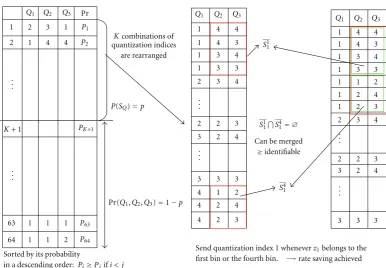
Simple example of merging process (3 nodes,Ri=2 bits)

Q1 Q2 Q3 Q1 Q2 Q3 _Q

1 Q2 Q3

Pr

1 2

2

2 2

2

2 2 2 2 2 2

2

2

2

2 3

3 3

3 3

3

3 3

3

3 3 3 3

3 3 3

3

3

3

3 3 3 3 1 P1

2 1 4 4

1 4

1 1

1

1 1 1

1 1 1

1 1

1 4

4

4

4 4 4

4

4

4

4 4

4

4 4

4

4

P2

. . .

. . .

. . .

. . . .

. . .

. .

K+ 1 PK+1

Pr(Q1,Q2,Q3)=1−p

63 1 1 1 P63

64 1 1 2 P64

Kcombinations of quantization indices

are rearranged

Can be merged

≥identifiable

Send quantization index 1 wheneverz1belongs to the first bin or the fourth bin. −→rate saving achieved Sorted by its probability

in a descending order: Pi≥Pjifi< j

S1

1

S1

1

∪

S4

1

S4

1

=∅

Figure3: Simple example of merging process, where there are 3 nodes and each node uses a 2 bit quantizer (Qi∈ {1, 2, 3, 4}). In this case, it is assumed that Pr(SM−SQ)=1−p≈0.

Definition 1. QijandQikare identifiable, and therefore can be

merged, if and only ifSij∩Ski = ∅.

Figure 3illustrates how to merge quantization bins for

a simple case, where there are 3 nodes deployed in a sensor field. It is noted that the first binQ11(equivalently,Q1 =1) and the fourth binQ41 at node 1 can be merged since the setsS1

1 andS41have no elements in common. This merging process will be repeated in the other nodes until there are no quantization bins that can be merged.

4. Quantization Schemes

As mentioned in the previous section, there will be redundancy in M-tuples after quantization which can be eliminated by our merging technique. However, we can also attempt to reduce the redundancy during quantizer design before the encoding of the bins is performed. Thus, it would be worth considering the effect of selection of a given quantization scheme on system performance when the merging technique is employed. In this section, we consider three schemes as follows.

(i) Uniform quantizers. Since they do not utilize any statistics about the sensor readings for quantizer design, there will be no reduction in redundancy by the quantization scheme. Thus only the merging technique plays a role in improving the system performance.

(ii) L1oyd quantizers. Using the statistics about the sensor readingziavailable at nodei, theith quantizerαiis designed

using the generalized L1oyd algorithm [16] with the cost function|zi−zi|2which is minimized in an iterative fashion.

Since each node consider only the information available to it during quantizer design, there will still exist much redundancy after quantization which the merging technique can attempt to reduce.

(iii) Localization specific quantizers (LSQs) proposed in [7].

While designing a quantizer at node i, we can take into account the effect of quantized sensor readings at other nodes on the quantizer design by introducing the localization error in a new cost function, which will be minimized in an iterative manner. (The new cost function to be minimized is expressed as the Lagrangian functional|zi−zi|2+λx−

x2_{. The topic of quantizer design in distributed setting} goes beyond the scope of this work. See [7,8] for detailed information.) Since the correlation between sensor readings is exploited during quantizer design, LSQ along with our merging technique will show the best performance of all.

We will discuss the effect of quantization and encoding on the system performance based on experiments for an acoustic amplitude sensor system inSection 9.1.

5. Proposed Encoding Algorithm

identifiable pairs cannot be merged simultaneously; that is, after a pair has been merged, other candidate pairs may become nonidentifiable. In what follows, we propose algorithms to determine in a sequential manner which pairs should be merged.

In order to minimize the total rate consumed by Mnodes, an optimal merging technique should attempt to reduce the overall entropy as much as possible, which can be achieved by (1) merging high probability bins together and (2) merging as many bins as possible. It should be observed that these two strategies cannot be pursued simultaneously. This is because high probability bins (under our assumption of uniform distribution of the source position) are large and thus merging large bins tends to result in fewer remaining merging choices (i.e., a larger number of identifiable bin pairs may become nonidentifiable after two large identifiable bins have been merged). Conversely, a strategy that tries to maximize the number of merged bins will tend to merge many small bins, leading to less significant reductions in overall entropy. In order to strike a balance between these two strategies, we define a metric, Wij, attached to each

quantization bin

Wij=P

j

i −γS

j

i, (7)

whereγ ≥0.This is a weighted sum of the bin probability and the number of the combinations of M-tuples that includeQij.IfP

j

i is large the corresponding bin would be a

good candidate for merging under criterion (1) whereas a small value of|Sij|will indicate a good choice under criterion

(2). In our proposed procedure, for a suitable value ofγ, we will seek to prioritize the merging of those identifiable bins having the largest total weighted metric. This will be repeated iteratively until there are no identifiable bins left. The selection ofγcan be heuristically made so as to minimize the total rate. For example, several different γ’s could be evaluated in (7) to first determine its applicable range which will be then searched to find a proper value ofγ.Clearly,γ

depends on the application.

The proposedglobal merging algorithmis summarized as follows.

Step 1. Set F(i,j) = 0, wherei = 1,. . .,M; j = 1,. . .,Li,

indicating that none of the bins,Qij, have been merged yet.

Step 2. Find (a,b) = arg max(i,j)|F(i,j)=0(Wij), that is, we

search over all the nonmerged bins for the one with the largest metricWb

a.

Step 3. FindQc

a,c /=bsuch thatWac =maxj=/b(W

j

a), where

the search for the maximum is done only over the bins identifiable with Qb

a at node a and go to Step 4. If there

are no bins identifiable withQb

a, setF(a,b)= 1, indicating

the binQb

a is no longer involved in the merging process. If F(i,j)=1, for alli,j, stop; otherwise, go toStep 2.

Step 4. MergeQb

aandQcatoQmin(a b,c)withSamin(b,c)=Sba∪Sca.

SetF(a, max(b,c))=1.Go toStep 2.

In the proposed algorithm, the search for the maximum of the metric is done for the bins of all nodes involved. However, different approaches can be considered for the search. These are explained as follows.

Method 1(Complete sequential merging). In this method, we process one node at a time in a specified order. For each node, we merge the maximum number of bins possible before proceeding to the next node. Merging decisions are not modified once made. Since we exhaust all possible mergers in each node, after scanning all the nodes no more additional mergers are possible.

Method 2(Partial sequential merging). In this method, we again process one node at a time in a specified order. For each node, among all possible bin mergers, the best one according to a criterion is chosen (the criterion could be entropy based and e.g., (7) is used in this paper) and after the chosen bin is merged we proceed to the next node. This process is continued until no additional mergers are possible in any node. This may require multiple passes through the set of nodes.

These two methods can be easily implemented with minor modifications to our proposed algorithm. Notice that the final result of the encoding algorithm will beMmerging tables, each of which has the information about which bins can be merged at each node in real operation. That is, each node will merge the quantization bins using the merging table stored at the node and will send the merged bin to the fusion node which then tries to determine which bin actually occurred via the decoding process usingM merging tables andSQ.

5.1. Incremental Merging. The complexity of the above procedures is a function of the total number of quantization bins, and thus of the number of the nodes involved. These approaches could potentially be complex for large sensor fields. We now show that incremental merging is possible; that is, we can start by performing the merging based on a subset consisting of N sensor nodes, N < M, and it can be guaranteed that the merging decisions that were valid whenNnodes were considered will remain valid even when all Mnodes are taken into account. To see this, suppose that Qij and Qik are identifiable when

only N nodes are considered. From Definition 1, Sij(N)∩ Sk

i(N) = ∅, where N indicates the number of nodes

involved in the merging process. Note that since every elementQj_{(M)=(Q1,. . .,Q}

N,QN+1,. . .,QM)∈Sij(M) (In

this section, we denote byQj_{(M) an element (Q1,. . .,Q}

i =

j,. . .,QM) ∈ Sij(M).Later, it will be also used to denote

an jth element in SQ in Section 8 without confusion) is constructed by concatenatingM−N indicesQN+1,. . .,QM with the corresponding element,Qj_{(N) = (Q1,. . .,Q}

N) ∈ Sij(N), we have thatQj(M)=/Qk(M) ifQj(N)=/ Qk(N).By

the property of the intersection operator ∩, we can claim thatSij(M)∩Sik(M)= ∅for allM ≥ N, implying thatQ

j

i

Thus, we can start the merging process with just two nodes and continue to do further merging by adding one node (or a few) at a time without change in previously merged bins. When many nodes are involved, this would lead to significant savings in computational complexity. In addition, if some of the nodes are located far away from the nodes being added (i.e., the dynamic ranges of their quantizers do not overlap with those of the nodes being added), they can be skipped for further merging without loss of merging performance.

6. Extension of Identifiability:

p

-Identifiability

Since for real operating conditions, there exist measurement noise (wi=/0) and/or parameter mismatches, it is

com-putationally impractical to construct the set SQ satisfying the assumption of Pr[Q ∈ SQ] = 1 under which the merging algorithm was derived in Section 3. Instead, we construct SQ(p) such that Pr[Q ∈ SQ(p)] = p( 1) and propose an extended version ofidentifiabilitythat allows us to still apply the merging technique under noisy situations. With this consideration, Definition 1 can be extended as follows.

Definition 2. Qij and Qki are p-identifiable, and therefore

can be merged, if and only if Sij(p)∩Ski(p) = ∅, where Sij(p) andSki(p) are constructed fromSQ(p) asS

j

i fromSQin

Section 2. Obviously, to maximize the rate gain achievable

by the merging technique, we need to construct SQ(p) as small as possible given p. Ideally, we can build the set

SQ(p) by collecting the M-tuples with high probability although it would require huge computational complexity especially when many nodes are involved at high rates. In this work, we suggest following the procedure stated below for construction ofSQ(p) with reduced complexity.

Step 1. Compute the intervalIzi(x) such thatP(zi∈Izi(x)| x) = p1/M _{= 1−β, for alli.Since z}

i ∼ N(fi,σi2), where

fi = f(x, xi,Pi) in (1), we can construct the interval

that is symmetric with respect to fi; that is, Izi(x) =

[fi−zβ/2 fi+zβ/2], so that

M

i Pr(zi ∈ Izi(x) | x) = p.

Notice thatzβ/2is determined byσiandβ(not a function of

x). For example, if (1−β) = 0.99, zβ/2 is given by 3σiand p=(1−β)M=0.95 withM=5.

Step 2. FromM intervals Izi(x),i = 1,. . .,M, we generate

possible M-tuples Q = [Q1,. . .,QM] satisfying that Qi

Izi= ∅/ , for alli.Denote bySQ(x) a set containing such M

tuples. It is noted that the process of generating M-tuples from M intervals is deterministic, given M quantizers. (Simple programming allows us to generate M-tuples from M intervals. For example, suppose that M = 3 and

Iz1 =[1.2 2.3], Iz2 =[2.7 3.3], andIz3 =[1.8 3.1] are computed given x inStep 1. Pick anM-tupleQ ∈ SMwith Q1 = [1.5 2.2], Q2 = [2.5 3.1], and Q3 = [2.1 2.8].

Then, we determine whether or not Q ∈ SQ(x) by checking Qi

Izi= ∅/ , for alli. In this example, we have

Q∈SQ(x).)

Step 3. Construct SQ(p) =

x∈SSQ(x).We have Pr(Q ∈

SQ(p))=Ex[Pr(Q ∈SQ(p)| x)] ≈Ex[

M

i Pr(zi ∈Izi(x)|

x)]=p.

Asβapproaches 1,SQ(p) will be asymptotically reduced to SQ, the set constructed in a noiseless case. It should be mentioned that this procedure provides a tool that enables us to change the size ofSQ(p) by simply adjustingβ.Obviously, computation of Pr(Q|x) is unnecessary.

Notice that all the merged bins are p-identifiable (or identifiable) at the fusion node as long as theM-tuple to be encoded belongs toSQ(p) (orSQ). In other words, decoding errors will be generated when elements inSM−SQ(p) occur and there will be tradeoffbetween rate savings and decoding errors. If we choose p to be as small as possible, yielding a small set SQ(p), we can achieve good rate savings at the expense of large decoding error (equivalently, Pr[Q∈SM−

SQ(p)] large), which could lead to degradation of localization performance. Handling of decoding errors will be discussed

inSection 7.

7. Decoding of Merged Bins and

Handling Decoding Errors

In the decoding process, the fusion node will first decom-pose the received M-tuple Qr into the possible M-tuples,

QD1,. . .,QDK by using theM merging tables (seeFigure 4). Note that the merging process is done offline in a centralized manner. In real operation, each node stores its merging table which is constructed from the proposed merging algorithm and used to perform the encoding and the fusion node uses

SQ(p) and M merging tables to do the decoding. Revisit the simple case inFigure 3. According to node 1’s merging table, Q11 and Q41 can be merged into Q11, implying that node 1 will transmit Q11 to the fusion node whenever z1 belongs toQ11orQ41.Suppose that the fusion node receives

Qr =(1, 2, 4).Then, it decomposes (1, 2, 4) into (1, 2, 4) and

(4, 2, 4) by using node 1’s merging table. This decomposition will be performed for the otherM−1 merging tables. Note that (1, 2, 4) is discarded since it does not belong toSQ(p), implying thatQ4

1actually occurred at node 1.

Suppose that we have a set of K M-tuples, SD =

{QD1,. . .,QDK}decomposed fromQrviaMmerging tables. Then, clearly, Qr ∈ SD and Qt ∈ SD, where Qt is the

trueM-tuple before encoding (seeFigure 4). Notice that if

Qt ∈ SQ(p), then all merged bins would be identifiable at the fusion node; that is, after decomposition, there is only one decomposed M-tuple, Qt belonging toSQ(p), (As the decomposition is processed, all the decomposed M-tuples except Qt will be discarded since they do not belong to SQ(p).) and we declare decoding successful. Otherwise, we declare decoding errors and apply the decoding rules which will be explained in the following subsections, to handle those errors. Since the decoding error occurs only when

Qt∈/ SQ(p), the decoding error probability will be less than 1−p.

It is observed that since the decomposed M-tuples are produced via theMmerging tables fromQt, it is very likely

f1 Q1 ENC

ENC

fM QM

Mencoders

x _{Z Q}

t QE Qr=QE .

. .

. . .

. . .

. . . Noiseless

channel

Recoding rule

decompo-sition via merging tables

QD

QD

1

QDK

One decoder at fusion node

Figure4: Encoder-decoder diagram: the decoding process consists of decomposition of the encodedM-tupleQE and decoding rule of computing the decodedM-tupleQDwhich will be forwarded to the localization routine.

In other words, since the encoding process merges the quantization bins whenever anyM-tuples that contain either of them are very unlikely to happen at the same time, theM -tuplesQDk (=/Qt) tend to take very low probability.

7.1. Decoding Rule 1: Simple Maximum Rule. Since the receivedM-tupleQrhas ambiguity produced by encoders at

each node, the decoder at fusion node should be able to find the trueM-tuple by using appropriate decoding rules. As a simple rule, we can take theM-tuple (out ofQD1,. . .,QDK) that is most likely to happen. Formally,

QD=arg max

k Pr

QDk

, k=1,. . .,K, (8)

whereQDis the decodedM-tuple which will be forwarded to

the localization routine.

7.2. Decoding Rule 2: Weighted Decoding Rule. Instead of choosing only one decoded M-tuple, we can treat each decomposed M-tuple as a candidate for the decoded M -tuple,QD with its corresponding weight obtained from the

likelihood. That is, we can viewQDkas one decodedM-tuple

with weight Wk = Pr[QDk]/

K

l Pr[QDl]k = 1,. . .,K. It

should be noted that the weighted decoding rule should be used along with the localization routine as follows:

x= K

k=1

xkWk k=1,. . .,K, (9)

where xk is the estimated source location assuming QD =

QDk.For simplicity, we can take a few dominantM-tuples

5 6 7 8 9 10 11 12 13 14 Total rate consumed by 5 nodes

0 2 4 6 8 10 12 14

A

ver

age

lo

calizat

ion

er

ro

r

(m

2)

UniformQ

LloydQ

LSQ

Figure 5: Average localization error versus total rate RM for three different quantization schemes with distributed encoding algorithm. Average rate savings is achieved by the distributed encoding algorithm (global merging algorithm).

for the weighted decoding and localization

x=

L

k

2 2.5 3 3.5 4 16

18 20 22 24 26 28 30 32 34 36

Number of bits assigned to each node,RiwithM=5

A

ver

at

e

rat

e

sa

ving

s

(a)

A

ver

at

e

rat

e

sa

ving

s

3 3.5 4 4.5 5

10 12 14 16 18 20 22 24 26 28

Number of nodes involved,

MwithRi=3 (b)

Figure6: Average rate savings achieved by the distributed encoding algorithm (global merging algorithm) versus number of bits,Riwith M=5 (left) and number of nodes withRi=3 (right).

whereW(k)is the weight ofQD(k) and Pr[QD(i)]≥ Pr[QD(j)] ifi< j.Typically,L(< K) is chosen as a small number (e.g.,

L=2 in our experiments). Note that the weighted decoding rule withL=1 is equivalent to the simple maximum rule in (8).

8. Application to Acoustic Amplitude

Sensor Case

As an example of the application, we consider the acoustic amplitude sensor system, where an energy decay model of sensor signal readings proposed in [4] is used for localization. The energy decay model was verified by the field experiment in [4] and was also used in [9,13,17].) This model is based on the fact that the acoustic energy emitted omnidirectionally from a sound source will attenuate at a rate that is inversely proportional to the square of the distance in free space [18]. When an acoustic sensor is employed at each node, the signal energy measured at node

i over a given time interval k, and denoted by zi, can be

expressed as follows:

zi(x,k)=gi a

x−xiα

+wi(k), (11)

where the parameter vector Pi in (1) consists of the gain

factor of the ith node gi, an energy decay factor α, which

is approximately equal to 2 in free space, and the source

signal energy a. The measurement noise term wi(k) can

be approximated using a normal distribution,N(0,σi2).In

(11), it is assumed that the signal energy, a, is uniformly distributed over the range [amin amax].

In order to perform distributed encoding at each node, we first need to obtain the setSQ, which can be constructed from (3) as follows:

SQ=

(Q1,. . .,QM)| ∃x∈S,Qi=αi

gi a

x−xiα+wi

,

(12)

where theith sensor readingzi(x) is expressed by the sensor

modelgi(a/x−xiα), and the measurement noise,wi.

When the signal energy a is known, and there is no measurement noise (wi=0), it would be straightforward to

construct the setSQ.That is, each element inSQcorresponds to one region in sensor field which is obtained by computing the intersection ofM ring-shaped areas (seeFigure 2). For example, using an j th elementQj _{=(Q1,. . .,Q}

M) inSQ, we can compute the corresponding intersectionAj_{as follows:}

Ai=

x|gi a

x−xiα ∈Qi, x∈S

, i=1,. . .,M,

Aj₌ M

i Ai.

40 50 60 70 80 90 100 SNR (Ri=3) withM=5

(σ=0.5) (σ≈0) 0

5 10 15 20 25 30 35

Rat

e

sa

vi

ng

s

(%)

Pr[decoding error]=0.0498

Pr[decoding error]=0.0202

Pr[decoding error]=0.0037

Rate savings (%) versus SNR whenRi=3 bits withM=5

Figure 7: Rate savings achieved by the distributed encoding algorithm (global merging algorithm) versus SNR (dB) withRi=3 andM=5. σ2_{=0,. . ., 0.5}2_.

Table1: Total rate,RMin bits (rate savings) achieved by various merging techniques.

Ri Method 1 Method 2 Method 3

2 9.4 (8.7%) 9.4 (8.7%) 9.10 (11.6%)

3 11.9 (20.6%) 12.1 (19.3%) 11.3 (24.6%)

4 13.7 (31.1%) 14.1 (29.1%) 13.6 (31.6%)

Since the nodes involved in localization of any given source generate the same M-tuple, the set SQ will be computed deterministically and we have Pr[Q∈SQ]=1.Thus, using

SQ, we can apply our merging technique to this case and achieve significant rate savings without any degradation of localization accuracy (no decoding error).

However, measurement noise and/or unknown signal energy will make this problem complicated by allowing random realizations of M-tuples generated byMnodes for any given source location. For this case, we constructSQ(p) by following the procedure in Section 6 and apply our decoding rules explained in Section 7 to handle decoding errors.

9. Experimental Results

The distributed encoding algorithm described inSection 5is applied to the system, where each node employs an acoustic amplitude sensor model given by (11) for source localization. The experimental results are provided in terms of average localization error. (Clearly, the localization error would be affected by the estimators employed at the fusion node. The estimation algorithms go beyond the scope of this work. For detailed information, see [9].)Ex−x2_{and rate savings (%)} computed by ((RT −RM)/RT)×100, where RT is the rate

Table2: Total rateRMin bits (rate savings) achieved by distributed encoding algorithm (global merging technique). The rate savings is averaged over 20 different node configurations, where each node uses LSQ withRi=3.

M Total rateRMin bits (rate savings)

12 17.3237 (51.56%)

16 20.7632 (56.45%)

20 23.4296 (60.69%)

consumed byMnodes when only the independent entropy coding (Huffman coding) is used after quantization and

RM is the rate by M nodes when the merging technique is applied to quantized data before the entropy coding. We assume that each node uses LSQ described inSection 4(for further details, refer to [7]) except for the experiments where otherwise stated.

9.1. Distributed Encoding Algorithm: Noiseless Case. It is assumed that each node can measure the known signal energy without measurement noise.Figure 5shows the over-all performance of the system for each quantization scheme. In this experiment, 100 different 5-node configurations were generated in a sensor field 10×10 m2_{.For each configuration,} a test set of 2000 random source locations was used to obtain sensor readings, which are then quantized by three different quantizers, namely, uniform quantizers, L1oyd quantizers, and LSQs. The average localization error and total rateRM are averaged over 100 node configurations. As expected, the overall performance for LSQ is the best of all since the total reduction in redundancy can be maximized when the application-specific quantization such as LSQ and the distributed encoding are used together.

Our encoding algorithm with the different merging techniques outlined inSection 5is applied for comparison, and the results are provided inTable 1. Methods 1 and 2 are as described inSection 5, and Method 3 is the global merging algorithm discussed in that section. We can observe that even with relative low rates (4 bits per node) and a small number of nodes (only 5) significant rate gains (over 30%) can be achieved with our merging technique.

The encoding algorithm was also applied to many dif-ferent node configurations to characterize the performance. In this experiment, 500 different node configurations were generated for eachM(=3, 4, 5) in a sensor field 10×10 m2_. The global merging technique has been applied to obtain the rate savings. In computing the metric in (7), the source distribution is assumed to be uniform. The average rate savings is plotted by varyingM andRiinFigure 6. Clearly,

the better rate savings is achieved with largerM and/or at higher rate since there exists more redundancy expressed as |SM−SQ|, as more nodes become involved at higher rate.

8.5 9 9.5 10 1.3

1.4 1.5 1.6 1.7 1.8 1.9 2 2.1

Total rate (bits) consumed by 5 sensors

Localization

er

ro

r

(m

2)

σ=0.05

σ=0

Ri=2

(a)

Total rate (bits) consumed by 5 sensors

Localization

er

ro

r

(m

2)

11.5 12 12.5 13 13.5 0.4

0.5 0.6 0.7 0.8 0.9 1 1.1

σ=0.05

σ=0

Ri=3

(b)

Figure8: Average localization error versus total rateRMachieved by the distributed encoding algorithm (global merging algorithm) with simple maximum decoding and weighted decoding, respectively. Total rate increases by changingpfrom 0.8 to 0.95 and weighted decoding is conducted withL=2.Solid line +: weighted decoding. Solid line +∇: simple maximum decoding.

is also the node density for the case ofM=5 in 10×10 m2_.

InTable 2, it is worth noting that the system with a larger

number of nodes outperforms the system with a smaller number of nodes (M = 3, 4, 5) although the node density is kept the same. This is because the incremental property of the merging technique allows us to find more identifiable bins at each node.

9.2. Encoding with p-Identifiability and Decoding Rules: Noisy Case. The distributed encoding algorithm with p -identifiability described inSection 6was applied to the case, where each node collects noise-corrupted measurements of unknown source signal energy. First, assuming known signal energy, we checked the effect of measurement noise on the rate savings, and thus the decoding error by varying the size ofSQ(p).Note that aspbecomes increased, the total rateRM tends to be increased since small rate gain is achieved with

SQ(p) large. In this experiment, the variance of measurement noise,σ2_{, varies from 0 to 0.5}2_{and for eachσ}2_{, a test set of} 2000 source locations was generated witha = 50.Figure 7 illustrates that good rate savings can be still achieved in a noisy situation by allowing small decoding errors. It can be noted that better rate savings can be achieved at higher SNR (Note that for practical vehicle target, the SNR is often much higher than 40 dB and a typical value of the variance of

measurement noiseσ2 _{is 0.05}2 _{[4,13].) and/or with larger} decoding errors allowed (Pr [decoding error]< 0.05 in this experiments).

For the case of unknown signal energy, where we assume thata∈[amin amax]=[0 100], we constructedSQ(p)= La

k=1SQ(ak) withΔa=ak+1−ak =(amax−amin)/La =0.5

by varying p = 0.8,. . ., 0.95, whereSQ(ak) is constructed whena=akusing the procedure inSection 6. UsingSQ(p), we applied the merging technique with p-identifiability to evaluate the performance (rate savings versus localization error). In the experiment, a test set of 2000 samples is generated from uniform priors for p(x) and p(a) with each noise variance (σ = 0 and 0.05). In order to deal with decoding errors, two decoding rules in Section 7 were applied. In Figure 8, the performance curves for two decoding rules were plotted for comparison. As can be seen, the weighted decoding rule performs better than the simple maximum rule since the former takes into account the effect of the other decomposedM-tuples on localization accuracy by adjusting their weights. It is also noted that when decoding error is very low (equivalently, p ≈ 1), both of them show almost the same performance.

8 9 10 11 12 13 14 15 16 Total rate consumed by 5 sensors

G1

G2

Ri=2

Ri=3

0.4 0.6 0.8 1 1.2 1.4 1.6 1.8 2 2.2

R-D w/o ENC forσ=0.05 R-D w/o ENC forσ=0

R-D w/ ENC forσ=0.05,p=0.85, 0.9, 0.95 R-D w/ ENC forσ=0,p=0.85, 0.9, 0.95

G1 Gain by ENC withσ=0.05,Ri=3 G2 Gain by ENC withσ=0,Ri=3

Localization

er

ro

r

(m

2)

Figure9: Average localization error versus total rate,RMachieved by the distributed encoding algorithm (global merging algorithm) withRi =3 and M = 5. σ = 0, 0.05. SQ(p) is varied from p = 0.85, 0.9, 0.95.Weighted decoding with L = 2 is applied in this experiment.

technique. InFigure 9, the performance curves (R-D curves) are plotted withp = 0.85, 0.9 and 0.95 forσ =0 and 0.05.

It should be noted that we can determine the size ofSQ(p) (equivalently, p) that provides the best performance from this experiment.

9.3. Performance Comparison. For the purpose of evaluation, it would be meaningful to compare our encoding technique with LSQ algorithm since both of them are optimized for source localization and can be viewed as DSC (distributed source coding) techniques which are developed as a tool to reduce the rate required to transmit data from all nodes to the sink. InFigure 10, the R-D curve for LSQ only (without our encoding technique) is plotted for comparison. It should be observed that at high rate, the encoding technique will outperform LSQ since the better rate savings will be achieved as the total rate increases.

We address the question of how our technique compares with the best achievable performance for this source localiza-tion scenario. As a bound on achievable performance we con-sider a system where (i) each node quantizes its measurement independently and (ii) the quantization indices generated by all nodes for a given source location are jointly coded (in our case, we use the joint entropy of the vector of measurements as the rate estimate).

Note that this is not a realistic bound because joint coding cannot be achieved unless the nodes are able to

8 10 12 14 16 18 20

0 0.5 1 1.5 2 2.5 3 3.5 4 4.5 5

A

ver

age

localization

er

ror

(m

2)

UniformQ+ ENC LSQ only

Total rate consumed by 5 sensors

Figure10: Performance comparison: Uniform quantizer equipped with distributed encoding algorithm versus LSQ only. Average localization error and total rate,RMare averaged for 100 different 5-node configurations.

communicate before encoding. In order to approximate the behavior of the joint entropy coder via DSC techniques one would have to transmit multiple sensor readings of the source energy from each node, as the source is moving around the sensor field. Some of the nodes could send measurements that are directly encoded, while others could transmit a syndrome produced by an error correcting code based on the quantized measurements. Then, as the fusion node receives all the information from the various nodes it would be able to exploit the correlation from the measurements and approximate the joint entropy. This method would not be desirable, however, because the information in each node depends on the location of the source and thus to obtain a reliable estimate of the measurement at all nodes one would have to have measurements at a sufficient number of positions of the source. Thus, instantaneous localization of the source would not be possible. The key point here, then, is that the randomness between measurements across nodes is based on the localization of the source, which is precisely what we wish to observe.

For a 5-node configuration, the average rate per node was plotted with respect to the localization error in Figure 11, with assumption of no measurement noise (wi = 0) and

Localization error (m2_),E(|x−x|2₎

0 0.2 0.4 0.6 0.8 1 1.2 1.4 1

2 3 4 5 6 7 8 9 10

A

ver

age

rat

e

(bits)

per

n

ode

UniformQ

LSQ

LSQ + distributed encoding UniformQ+ joint entropy coding LSQ + joint entropy coding

Rate savings achieved by distributed encoding algorithm

Figure 11: Performance comparison: distributed encoding algo-rithm is lower bounded by joint entropy coding.

10. Conclusion and Future Works

Using the distributed property of the quantized sensor readings, we proposed a novel encoding algorithm to achieve significant rate savings by merging quantization bins. We also developed decoding rules to deal with the decoding errors which can be caused by measurement noise and/or parame-ter mismatches. In the experiment, we showed that the sys-tem equipped with the distributed encoders achieved signif-icant data compression as compared with standard systems.

So far, we have considered encoding algorithms by fixing quantizers. However, since there exists dependency between quantization and encoding of quantized data which can be exploited to obtain better performance gain, it would be worth considering a joint design of quantizers and encoders.

Acknowledgments

The authors would like to thank the anonymous reviewers for their careful reading of the paper and useful suggestions which led to significant improvements in the paper. This research has been funded in part by the Pratt & Whitney Institute for Collaborative Engineering (PWICE) at USC, and in part by NASA under the Advanced Information Sys-tems Technology (AIST) program. The work was presented in part in IEEE International Symposium on Information Processing in Sensor Networks (IPSN), April 2005.

References

[1] F. Zhao, J. Shin, and J. Reich, “Information-driven dynamic sensor collaboration,” IEEE Signal Processing Magazine, vol. 19, no. 2, pp. 61–72, 2002.

[2] J. C. Chen, K. Yao, and R. E. Hudson, “Source localization and beamforming,”IEEE Signal Processing Magazine, vol. 19, no. 2, pp. 30–39, 2002.

[3] D. Li, K. D. Wong, Y. H. Hu, and A. M. Sayeed, “Detection, classification, and tracking of targets,”IEEE Signal Processing Magazine, vol. 19, no. 2, pp. 17–29, 2002.

[4] D. Li and Y. H. Hu, “Energy-based collaborative source local-ization using acoustic microsensor array,”EURASIP Journal on Applied Signal Processing, vol. 2003, no. 4, pp. 321–337, 2003. [5] J. C. Chen, K. Yao, and R. E. Hudson, “Acoustic source

localization and beamforming: theory and practice,”EURASIP Journal on Applied Signal Processing, vol. 2003, no. 4, pp. 359– 370, 2003.

[6] J. C. Chen, L. Yip, J. Elson et al., “Coherent acoustic array processing and localization on wireless sensor networks,”

Proceedings of the IEEE, vol. 91, no. 8, pp. 1154–1161, 2003. [7] Y. H. Kim and A. Ortega, “Quantizer design for source

localization in sensor networks,” inProceedings of the IEEE International Conference on Acoustics, Speech, and Signal Processing (ICASSP ’05), pp. 857–860, March 2005.

[8] Y. H. Kim,Distrbuted algorithms for source localization using quantized sensor readings, Ph.D. dissertation, USC, December 2007.

[9] Y. H. Kim and A. Ortega, “Maximum a posteriori (MAP)-based algorithm for distributed source localization using quantized acoustic sensor readings,” in Proceedings of the IEEE International Conference on Acoustics, Speech and Signal Processing (ICASSP ’06), pp. 1053–1056, May 2006.

[10] Y. H. Kim and A. Ortega, “Quantizer design and distributed encoding algorithm for source localization in sensor net-works,” inProceedings of the 4th International Symposium on Information Processing in Sensor Networks (IPSN ’05), pp. 231– 238, April 2005.

[11] T. J. Flynn and R. M. Gray, “Encoding of correlated observa-tions,”IEEE Transactions on Information Theory, vol. 33, no. 6, pp. 773–787, 1988.

[12] P. Ishwar, R. Puri, K. Ramchandran, and S. S. Pradhan, “On rate-constrained distributed estimation in unreliable sensor networks,”IEEE Journal on Selected Areas in Communications, vol. 23, no. 4, pp. 765–774, 2005.

[13] J. Liu, J. Reich, and F. Zhao, “Collaborative in-network processing for target tracking,”EURASIP Journal on Applied Signal Processing, vol. 2003, no. 4, pp. 378–391, 2003. [14] H. Yang and B. Sikdar, “A protocol for tracking mobile targets

using sensor networks,” inProceedings of IEEE Workshop on Sensor Network Protocols and Applications (SNPA ’03), pp. 71– 81, Anchorage, Alaska, USA, May 2003.

[15] T. M. Cover and J. A. Thomas,Elements of Information Theory, Wiley-Interscience, New York, NY, USA, 1991.

[16] K. Sayood,Introduction to Data Compression, Morgan Kauf-mann Publishers, San Fransisco, Calif, USA, 2nd edition, 2000. [17] A. O. Hero III and D. Blatt, “Sensor network source localiza-tion via projeclocaliza-tion onto convex sets (POCS),” inProceedings of the IEEE International Conference on Acoustics, Speech, and Signal Processing (ICASSP ’05), pp. 689–692, March 2005. [18] T. S. Rappaport,Wireless Communications:Principles and