Green's Tensor and 2Dimiensional BIE Method in Static
of Massif with Arbitrary Anisotropy
Sh. A. Dildabayev
*, G. K. Zakir’yanova
Institute of Mechanics and Engineering, Kazakhstan
*
Corresponding Author: [email protected]
Received August 30, 2019; Revised October 12, 2019; Accepted October 19, 2019
Copyright©2019 by authors, all rights reserved. Authors agree that this article remains permanently open access under the terms of the Creative Commons Attribution License 4.0 International License
Abstract
Up to now remains open the question of constructing fundamental solutions of the two-dimensional statics of an elastic body with arbitrary anisotropy. Also in the scope of BEM method, the question of calculating stresses in boundary points and points located close to the boundary of the region still remains actual. In this work, fundamental solutions of the static problem for elastic plane with arbitrary anisotropic properties are obtained as the sum of residues with complex variable function. The assessments of fundamental solution and theirs derivatives are presented in closed form. In the distribution space obtained are the regular representations for the Somigliana formulas and the stress calculation formulas. The numerical implementation of the BIE method in direct formulation has been realized in standard way. The test results performed for circular hole in anisotropic plane of rhombic system show a higher compliance with the boundary values of displacements and stresses and with nodes placed close to boundary. The results of analysis of the stress-strain state in the vicinity of rectangular mining chambers located deep from day surface are presented in tables and pictures of isolines.Keywords
Elastic, Anisotropy, Interior, Exterior, Boundary Value Problem, Distributions, Singular, Regular, Fundamental Solution, Convolution, Stress, Mining Chamber, Pillar1. Introduction
The construction of fundamental solution and BEM implementation mainly for orthotropic plane domain were considered in [1-7]. Fundamental solutions for transversely isotropic magneto-electro-elastic media and boundary integral formulation where provided in [8]. The questions of justification of BEM for infinite domains were discussed in [10] for isotropic media and in [11] for orthotropic
media. In [12] described the transformation technique of weakly singular and hyper singular integrals over arbitrary convex polygon into the regular contour integrals that can be easily calculated analytically or numerically.
This work is intended to show the technique to construct the fundamental solution for elastic plane with arbitrary anisotropic properties and demonstrate the ways to obtain the regular representation of singular integrals usually take place in practice of BEM method usage.
1.1. Statement of Problem
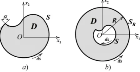
Let’s consider the domain D in plane R2 bounded by contour S, the contour may have corner nodes. For the interior problem we will consider simply connected domain inside the contour S (Fig. 1a). For exterior problem we will consider the doubly connected domain placed outside of S (Fig. 1b), where circle SR with radius R and center at O is sufficiently large so that the region bounded by SR covers S. In case of R→∞ we will have infinite domain with internal boundary S. Hereafter the unit outer normal is denoted by n.
Figure 1. Interior A) And Exterior B) Problem Domains.
The differential equation of equilibrium state for homogenous anisotropic elastic body, occupied domain D, has the next form [13]
, 2 , 1 , , , , ,
0 ) ( ) (
, +F = ∈D i j k l=
u
[image:1.595.310.534.560.675.2]where ui(x) are the components of displacement vector u in point x=(x1,x2), Fi(x) are body force components, {Eijkl} are matrix of elasticity constants with next symmetry property Eijkl= Ejikl = Eijlk= Eklij. According to index notation the indices after comma denotes the second derivatives with respect to spatial variable xl and xj, and repeated index denotes summation.
The symmetry property lets present {Eijkl} matrix as 6
×
6 matrix Eαβ (α,β=1,..,6). The relationship between pairs of (ij), (ml) indices and α,β indices established by next scheme (11) ↔ 1, (22) ↔ 2, (33) ↔ 3, (23)=(32)↔4, (31)=(13) ↔ 5, (31)=(13) ↔ 5.The first and the second boundary-value problem of plane-strain elasticity is posed as follows.
Find uϵ C2 (D) ∩C1 (S) such that (1) is satisfied in the domain D with given values of boundary displacement fi(x) or boundary loading gi(x):
2 , 1 , ), ( )
( = f ∈S i=
ui x i x x , (2)
2
,
1
,
),
(
)
(
)
(
,
n
=
g
∈
S
i
=
u
E
ijkl klx
jx
ix
x
. (3)2. Somigliana Formulas in Distribution
Space
2.1. Basic Equation in Distributions Space
Hereafter introduce abbreviations BVP1 and BVP2 for boundary value problem (1, 2) and (1, 3) consequently. For getting solution of BVP1 and BVP2 extend functions trough all plane R2 by entering distributions in accordance with [14] ), ( ) ( ) ( ˆ ), ( ) ( ) ( ˆ x x x x x x i D i i D i F H F u H u = = (4)
where HD(x) is the characteristic function of domain D. Its value in Rn (n=1,2,…) we determine according to [15]
∉ ∈ ∈ = = → . , 0 , ) 2 /( , , 1 ) ( )) ( ( lim ) ( 0 D S D S S D HD x x x x
x α π
m m
ε ε ε
(5)
Here Sε(x) is a sphere in Rn (ring for n=2) with radius ε and center in point x, m(•)- is volume (square) of region, α is an value of solid angle, formed by all kinds of tangent planes in boundary point x (Fig.1.a). The definition of HD(x) given by (5) makes possible to determine its value not only for interior and exterior points, but also for boundary points. For points on smooth part of boundary in Rn we always have HD(x)=0.5, for points on the corner of rectangular hole in R2 HD(x)=0.25. So the characteristic function is always a number.
The distributions given by (5) are equal to ui(x) and Fi(x) inside of D end equal to zero outside of D. Calculation second derivatives of with respect to spatial variables gives us next:
(
( ))
( ) ( ),) ( )
(
ˆi,kj x njui,k x S j nkui x S ui,kj x HD x
u =−
δ
−∂δ
+(6)
here и are consequently well
known single layered and double layered potential distributions on contour S [14]. By using (6) we can get next expression for generalized equilibrium equation
(
( ))
. ) ( ) ( ˆ ) (ˆk,lj i ijkl j k,l S ijkl j l k S
ijklu F E n u E nu
E x + x =− xδ − ∂ xδ
(7) So from solving of BVP1 or BVP2 we come to find the generalized solution in D of equations (7). Solution of equation (7) in view of its definition by (4) coincides in D with solution of BVP1 or BVP2.
2.2. Green Tensor and Other Fundamental Solutions
To obtain fundamental solution of differential equations (1) we let body force component to be Fi(x)= δiβδ(x), that represent concentrated force acting in xβ direction and applied in point x, here δiβ and δ(x) are Kronecker– delta and Dirac–delta. The solution for this force is entitled as Green tensor and be denoted as Uiβ(x). To construct the Green's tensor, it is convenient to use the Fourier transform, which brings the system (1) to the next system of linear equation in transform space
β
β ω ω δ
ω
ωj l kF i
ijkl U i i
E ( 1, 2)= , (8) here ωi is Fourier transform parameter. The solution of system (8) give us
) , ( ) , ( ) , ( 2 1 2 1 2
1 ω ω
ω ω ω ω β β Q Q i i
UkF = k , (9)
here Q(ω1, ω2) is uniform polynomial of degree 4 and represent the determinant of system (8), Qkβ(ω1, ω2) are uniform polynomials of degree 2 and
). , ( ) , ( ) , ( ) , ( , 2 ) , ( , ) ( ) , ( , 2 ) , ( 2 1 2 12 2 1 12 2 1 12 2 1 2 2 66 2 1 16 2 1 11 2 1 22 2 2 26 2 1 66 12 2 1 16 2 1 12 2 2 22 2 1 26 2 1 66 2 1 11 ω ω ω ω ω ω ω ω ω ω ω ω ω ω ω ω ω ω ω ω ω ω ω ω ω ω Q Q Q Q E E E Q E E E E Q E E E Q − = + + = − + − − = + + = (10)
By using inverse Fourier transform formula we will obtain Green’s tensor in Cartesian Ox1x2 coordinates
2 1 2
0 0 1 2 2 1 2 2 2 1 1 ) , ( ) , ( 4 1 )
( ω ω
ω ω ω ω π ω ω π d d e Q Q
Ukj kj −ix −ix
∞
∫∫
=
x
Next proceed to polar coordinates ω1=rcosα, ω2=rsinα and using uniformity of polynomials we can get
∫
∫∫
+ − = = = − + ∞ π α α ρ π α α α α α α α π α ρ α α ρ α α π 2 0 2 1 2 ) sin cos ( 2 0 0 2 ) sin cos ln( ) sin , (cos ) sin , (cos 4 1 ) sin , (cos ) sin , (cos 4 1 )( 1 2
d x x Q Q d d e Q Q U kj x x i kj kj x ) ( ˆ ), ( ˆi x Fi x
u ) ( ˆ x u S k i ju
n , (x)
δ
∂j(
nkui(x)δ
S)
) ( ˆi x
In last by introducing variable transformation z= ctgθ we obtain
∫
∞ ∞ − + − − − + −= x z x z dz
z z Q z z Q z
Ukj kj 2
2 1 2 2 2 2 2 ) 1 ( ln ) 2 , 1 ( ) 2 , 1 ( ) 1 ( 2 1 ) ( π x
According to the complex function theory the last integral is equal to sum of restudies of it integrand
[
( 1)/2]
}
.ln ) 2 , 1 ( ) 2 , 1 ( ) 1 ( 1 ) ( 2 2 1 2 2 2 8 1Im 0
2 p p
p p p p ki p p z
ki x z x z
z z Q z z Q z res U p + − × − − + − =
∑
= > πx (11)
here zp (p=1,…,8) are the roots of polynomial Q(z) of degree 8 and in calculation are used only those that are placed in upper half plane of complex variable z. In view of logarithm is multivalued function it is necessary to remain on the same branch when traversing zeros of an expression in complex plane z
. 0 2 / ) 1 ( 2 2
1 zp− +x zp =
x
Notice that the root values of polynomial Q(z) in view of (10) depend only on the elastic constants. In view of this matter, it is easy to obtain other fundamental solutions which are the derivatives of Green tensor with respect to spatial variables: , ) 2 , 1 ( ) 2 , 1 ( ) 1 ( 2 / ) 1 ( 2 / ) 1 ( 1 ) ( 2 2 2 2 2 1 2 2 1 8
1Im 0 2 , − − + × + − + − − =
∑
= > p
p ki p p l p l p z l ki z z Q z z Q z z x z x z z res U p δ δ π
x (12)
[
][
]
[
]
+ − + − + − × − − + − =∑
= > ( 1)/2
2 / ) 1 ( 2 / ) 1 ( ) 2 , 1 ( ) 2 , 1 ( ) 1 ( 1 ) ( 2 2 2 1 2 2 1 2 2 1 2 2 2 8 1Im 0 2 , p p p j p j p l p l p p p p ki p z lj ki z x z x z z z z z z Q z z Q z res U p δ δ δ δ π x
For assessment of Green tensor and its derivatives, it is useful to present them in next form:
[
cos ( 1)/2 sin]
, ln ) 2 , 1 ( ) 2 , 1 ( ) 1 ( ln ) ( 2 2 2 2 8 1Im 0 2 + − − − + − =∑
= > p p p p p p ki p zki z z
z z Q z z Q z res r U p θ θ π x , ) 2 , 1 ( ) 2 , 1 ( ) 1 ( sin 2 / ) 1 ( cos 2 / ) 1 ( 1 2 2 2 2 2 2 1 8
1Im 0 2 , − − + × + − + − − =
∑
= > p
p ki p p l p l p z l ki z z Q z z Q z z z z z res r U
p θ θ
δ δ π
[
][
]
[
]
+ − + − + − × − − + − =∑
= > 2 2
2 2 1 2 2 1 2 2 2 8 1Im 0 2 2 , sin 2 / ) 1 ( cos 2 / ) 1 ( 2 / ) 1 ( ) 2 , 1 ( ) 2 , 1 ( ) 1 ( 1 p p p j p j p l p l p p p p ki p z lj ki z z z z z z z z Q z z Q z res r U
p
θ
θ
δ
δ
δ
δ
π
(13). / sin , / cos
, 1 2
2 2 2
1 x x r x r
x
r= + θ= θ =
According to (13) for any direction {cosθ, sinθ} on plane R2 we have next assessments for behavior of Green tensor and its derivatives when r →∞ or r →0
2 , ,( ) , ( ) , | ln | ) ( r C U r B U r A
Ukβ x ≤ kβl x ≤ kβlj x ≤ (14) here A, B, C are some real positive constants.
2.3. Somigliana and Stress Formulas in Distributions Space
[
]
. , ) ( ) , ( ) ( ) , ( ) ( ) , ( ) , ( ˆ D dV F U dS u T p U t u y D k ki y S k ki k ki i ∈ + + − =∫
∫
x y y x y y x y y x x (15)In (15) we introduce next designations
), ( ) ( )
(x k,j x j x
k u n
p = (16)
1 11 1 ,1 12 2 ,3 16 1 ,2 2 ,1 1 16 1 ,1 36 2 ,2 66 1 ,2 2 ,1 2 2 16 1 ,1 26 2 ,2 66 1 ,2 2 ,1 1 12 1 ,1 22 2 ,2 36 1 ,2 2 ,1 2
(
)
(
)
,
(
)
(
)
,
i i i i i i i i i
i i i i i i i i i
T
E U
E U
E U
U
n
E U
E U
E
U
U
n
T
E U
E U
E
U
U
n
E U
E U
E
U
U
n
=
+
+
+
+
+
+
+
=
+
+
+
+
+
+
+
(17)here pk are component of boundary loading, and Tkβ are fundamental traction tensor components generated by Green tensor, nk components of outer normal. In view of (17) fundamental traction tensor is not symmetric tensor.
In (15) the generalized displacement in any point of D, exclude contour S, expressed by sum of integral of single layered potentials of boundary loading values pk, double layered potential of boundary displacement values uk and Newton potential of body force Fk.
Formula (15) is obtained for distributions. Note that in (15) on the right and on the left there are regular generalized functions for xϵD. From du Bois-Reymond’s Lemma [14], it is known that every locally integrable function f defines a regular generalized function by the formula (f, ϕ) (ϕ - from the space of basic functions and contrary every regular distribution is defined by a unique locally integrable function. Due to this equation (15) are also valid in the usual sense. Similar formula for elastic media usually is obtained using Betty's theorem of the elasticity theory. The approach based on the use of distributions and performed here is more correct, since the fundamental solutions are singular distributions and to work with them it is necessary to use the same space of functions in which they are defined.
By derivation displacement given by (13) with respect to spatial variable xi and using the elasticity Hook’s law the stress formulae is obtained
[
D p V u]
dS W F dVy DD i ikm S y i ikm i ikm
km(x)=
∫
(x,y) (y)− (x,y) (y) +∫
(x,y) (y) , x∈σ (18)
where potentials kernel are
(
)
(
)
(
)
,. , , 1 , 2 2 , 1 66 2 , 2 26 1 , 1 16 21 1 , 2 2 , 1 26 2 , 2 22 1 , 1 12 22 1 , 2 2 , 1 16 2 , 2 12 1 , 1 11 11 i i i i i i i i i i i i i i i U U E U E U E D U U E U E U E D U U E U E U E D + + + = + + + = + + + = (19)(
)
(
)
(
)
,. , , 1 , 2 2 , 1 66 2 , 2 26 1 , 1 16 21 1 , 2 2 , 1 26 2 , 2 22 1 , 1 12 22 1 , 2 2 , 1 16 2 , 2 12 1 , 1 11 11 i i i i i i i i i i i i i i i T T E T E T E V T T E T E T E V T T E T E T E V + + + = + + + = + + + = (20)(
)
(
)
(
)
,. , , 1 , 2 2 , 1 66 2 , 2 26 1 , 1 16 21 1 , 2 2 , 1 26 2 , 2 22 1 , 1 12 22 1 , 2 2 , 1 16 2 , 2 12 1 , 1 11 11 i i i i i i i i i i i i i i i U U E U E U E W U U E U E U E W U U E U E U E W + + + = + + + = + + + = (21)So the Somigliana formula give the solution of BVP1 or BVP2 thereat for BVP1 we have Fredholm equations of first kind, and second kind for BVP2 when xϵS.
2.4. Gauss Formula and Regular Presentation of Somigliana and Stress Formulas
In view of assessments (14), for Green tensor and its derivatives, the potential kernels Tiβ(x,y) in Somigliana formulas and potential kernels Dikj(x,y), Vikj(x,y) has singularities on contour S when x=y. For performing, the regular presentation of (14) is used Gauss formula for double-layered potential. In this objection, lets take convolution of characteristic function HD(x) (5) of finite domain D with equilibrium equation for concentrated body force
. , 0 ) ( ) ( 2 , R U
Performing convolution with first term gives
) ( )
( )
( ) ( )
( )
( )
( , ,
, 2
x y
x y
y x y
x x
y
x β β β β
β y i
S i y j
S
l k ijkl y
D
lj k ijkl y
R
D lj
k
ijklU H dV E U dV E U n dS T dS T
E − =
∫
− =∫
− =∫
− =∫
In last expression on pass from body integral to contour integral the Gauss formula is used. Convolution with second terms gives
) ( )
( )
( ) (
2
x y
x y
x
x y i D
D i y i
R
D dV dV H
H δβδ − =δβ
∫
δ − =δβ∫
Finally, for double potential kernel Tiβ we obtain the Gauss formulas for finite domain D with finite contour )
( )
, ( )
(x x y y i D x
S i
i T dS H
T β =
∫
β =−δβ (21)For infinite domain consider the doubly connected domain D placed outside of S (Fig. 1b), where circle SR with finite radius R with center at O is sufficiently large so that the region bounded by SR covers S. For this finite domain we have
) ( )
, ( )
(x x y y i D x
S S
i
i T dS H
T
R
β β
β =
∫
=−δ
∪
or
) ( )
, ( )
,
(x y x y y i D x
S i y
S
i dS T dS H
T
R
β β
β +
∫
=−δ
∫
For finite contour SR with arbitrary large radius R integral of double potential with kernel Tiβ in view of (21) is equal to –δiβHD(x) and we have
) ( )
( )
,
(x y y i D x i D x
S
i dS H H
Tβ −δβ =−δβ
∫
And as the last equality is valid for arbitrary contour of large diameter R so it also valid for R→∞ and finally we have Gauss formula for infinite domain outside of S
, )) ( 1 ( ) , ( )
( β β
β y D δi
S i
i T dS H
T x =
∫
x y = − x (22)Gauss formula is important in applications because it gives simply and obvious geometric representation to get the values of double layered potential of fundamental traction tensor and to verify its numerical implementation. The direct numerical calculations for Gauss formulae were implemented and the results are presented in next section.
Using Gauss formulae we can obtain the regular representation of Somigliana formulas. By adding to (15) Gauss formulas (21) multiplied on uk(x) in case when xϵD we have next expression
(
1 H ( ))
u( ){
U ( , )p ( ) T ( , )(
u ( ) u ( ))
}
dS U ( , )F ( )dVy, x D.D
k ki y
S
k k ki k ki i
D = − − + ∈
− x x
∫
xy y xy y x∫
xy y (23)In view definition (5) of HD(x) the left side of (23) for interior BVP equal to zero and for exterior problems the left side is equal to uβ(x). In this representation when integration point y is very close to x (x in domain or on contour) we have integrable singularity.
In case xϵS the expression (23) becomes boundary integral equation (BIE), and exclusion of singularity in this manner is very useful during numerical solution of BIE.
By derivation displacement given by (23) with respect to spatial variable xi and using Hook’s law the regular representation of stress formulae is obtained
(
)
[
]
. , ) ( ) , ( )
, ( ) (
) ( ) ( ) , ( ) ( ) , ( )
(
D dV
F W
dS T
dS u u V
p D
y
D
i ikq y
S i iq S
y k k ikq
i ikq kq
∈ +
+
+ −
− =
∫
∫
∫
x y
y x y
x x
x y y x y
y x x
β σ
σ
(24)
[
(
( ) ( ))
]
( , ) ( ) , , ) , ( ) ( ) , ( ) 2 /( ) ( 1 1 ) ( S dV F W dS u u V p D H y D i ikm y k k ikm S i ikm D km ∈ + − × × − + − =∫
∫
x y y x x y y x y y x x x π α σ (25)where HD(x) = 1 for interior BVP of finite regions, and HD(x) = 1 for exterior BVP of infinite domain.
3. Numerical Implementation and Test
Results
3.1. Discrete Analogues of Somigliana and Stress Formulas
The numerical implementation of the BIE method in direct formulation has been realized in standard way. The boundary contours of region were approximated by the finite set of {Sl} (l = 1, L) of 3-nodal isoperimetric quadrilateral elements (See Fig 2.). The nodes of all elements and regional nodes form some finite set of nodes ordered by continuous numbering. In accordance with this, each boundary node will have a unique global number in set and local number on element. In follows we will use upper indexing for the node values of the desired and given functions fik = fi(xk).
Figure 2. 3-Nodal Quadrilateral Isoperimetric Element
The Cartesian coordinates yi of an arbitrary point of the element Sk, and the values of the functions at this point are parametrically expressed in terms of the node values using the form functions of the local coordinates ζ=(ζ1, ζ2) in form of relations:
∑
∑
= = ≤ = ≤ = 3 1 ) , ( 3 1 ) , ( , 1 | | , ) ( ) ( , 1 | | , ) ( ) ( k k l i k i k k l i k i f L f y L y ξ ξ ξ ξ ξ ξ ϕ ϕ (26)here ϕ(l,k) is the global number of the node having the local number k in the l–th element, Lk(ξ) are form-functions of isoperimetric element ). 1 ( 5 . 0 ) ( ), 1 )( 1 ( ) ( ), 1 ( 5 . 0 ) ( 3 2 1 + = − + − = − = ξ ξ ξ ξ ξ ξ ξ ξ ξ L L L (27)
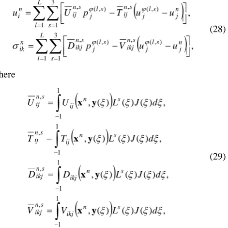
The discrete analogues of regularized boundary integral equation (23) and stress formulae’s (25) in assumption of absence of body force are obtained by replace contour integral by sum of integral on the elements and using interpolation (26) and form-functions(27)
(
)
(
)
, , 1 3 1 ) , ( , ) , ( , 1 3 1 ) , ( , ) , ( ,∑∑
∑∑
= = = = − − = − − = L l s n j s l j s n ikj s l j s n ikj n ik L l s n j s l j s n ij s l j s n ij n i u u V p D u u T p U u ϕ ϕ ϕ ϕ σ (28) here(
)
(
)
(
)
(
, ( ))
( ) ( ) , , ) ( ) ( ) ( , , ) ( ) ( ) ( , , ) ( ) ( ) ( , 1 1 , 1 1 , 1 1 , 1 1 , ξ ξ ξ ξ ξ ξ ξ ξ ξ ξ ξ ξ ξ ξ ξ ξ d J L V V d J L D D d J L T T d J L U U s n ikj s n ikj s n ikj s n ikj s n ij s n ij s n ij s n ij∫
∫
∫
∫
− − − − = = = = y x y x y x y x (29)J(ξ) is the Jacobean of the transformation (26). The integrals (29) are calculated by using Gauss quadrature.
In case when the element Sl includes node xn it subdivided on subelements according to technique suggested in [16].
For calculation roots of polynomials Q(z2+1, 2z) the Newton method was performed.
3.2. Compare with Analytical Solution for Exterior Problem of Infinite Domain
For verification of proposed fundamental solution and regular representation of Somigliana and stress formulas the numerical results were compared with analytical solution given in [13] for cylindrical hole with unit radius R=1 under inner pressure. Anisotropic media of rhombic system (aragonite (CaCO3)) [17] is considered with elastic constants
[image:6.595.305.541.235.470.2](30) are given for the case when the directions of the principal axes of symmetry of the elastic constants coincide with the directions of the axes of global system coordinates. Next, on occasion, for indexed coordinates xi (i=1,2,3) we use traditional symbols x, y and z consequently.
In case when the direction of global axes coordinate Oxyz and the directions of symmetry axes of elastic constants Oξνζ are differ, the elastic constant values in global coordinate system are expressed by
ijkl ls kr jq ip
pqrs C
C =
α
α
α
α
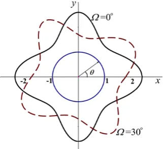
′ (31) here Cijlk′ – elastic constant values in principal symmetry axes, αij-direction cosines of principal symmetry axes in global system. In the case of two-dimensional problems, it is possible only the axes rotation in the Oxy plane relative to the origin. The rotation angle of the axes of the Oξν system relative to the Oxy axes will be denoted by Ω.The numerical results are computed by solving integral equation (23) and stress calculation by (24,25) for approximation of hole with 16 and 32 of 3-nodal isoperimetric elements.
The epure of obtained circular σθ stress in case Ω= 0° is symmetrical about axe Oy (see Fig.2) and σθ values are equal to 1.4530 at θ= 0°, and 1.6206 at θ= 90°. In case Ω= 30° the epure of σθ stress rotated by 30°.
Figure 3. Circular σθ stresses distribution on contour of cylindrical hole for Ω= 0° and 30°.
Below in Table 1 are presented numerical and analytical results of radial displacements uR and circular stresses σθ for Ω=0° in some boundary and regional nodes, placed close to hole contour on radiuses 1.005, 1.01, 1.02, 1.1 in case of contour division by L=16 and L=32 elements.
The obtained numerical results are in good agreement with analytical values even for so rough approximation of boundary contour. The numerical boundary stress values are in conform to those analytical better than the stress values for regional nodes placed concentering on radius r=1.005 and r=0.01. This indicates the extra high efficiency of calculation boundary displacement and stress values using regular representation for Somigliana (23) and stress (26) formulas.
Table 1. Comparison of numerical and analytical radial displacement ur
and angular stress σθ values in boundary and regional points
x y ur L=16 uran σθ L=16 σθ L=32 σθan
1.000 0.000 1.0160 1.0167 1.4530 1.4410 1.4393
0.924 -0.383 1.1437 1.1445 0.9982 0.9951 0.9946
0.707 -0.707 1.4050 1.4058 0.5982 0.6007 0.6010
0.000 -1.000 1.7077 1.7085 1.6206 0.1605 1.6027
1.005 0.000 1.0267 1.0135 1.3901 1.4063 1.4074
0.928 -0.385 1.1946 1.1372 0.6869 0.9611 0.9878
0.711 -0.711 1.4023 1.3970 0.5682 0.6197 0.6039
0.000 -1.005 1.7451 1.7026 1.5027 1.5478 1.5485
t1.010 0.000 1.0244 1.0103 1.3764 1.3766 1.3769
0.933 -0.387 1.1207 1.1301 0.9621 0.9813 0.9807
0.714 -0.714 1.3836 1.3882 0.6213 0.6072 0.6067
0.000 -1.010 1.7023 1.6967 1.4973 1.4982 1.4986
1.020 0.000 0.9857 0.9862 1.3192 1.3195 1.3196
0.942 -0.390 1.0772 1.0778 0.9666 0.9659 0.9660
0.721 -0.721 1.3194 1.3200 0.6125 0.6119 0.6119
0.000 -1.020 1.6514 1.6519 1.4084 1.4089 1.4092
1.100 0.000 0.9581 0.9586 0.9886 0.9888 0.9890
1.016 -0.421 1.0210 1.0215 0.8387 0.8389 0.8390
0.778 -0.778 1.2396 1.2401 0.6363 0.6364 0.6365
0.000 -1.100 1.5998 1.6003 0.9768 0.9772 0.9774
[image:7.595.306.536.100.406.2]The results of direct numerical calculation of double potential integral Tij(x) (22) for Ω=0° in case of circular contour division by 16 elements for some boundary and regional nodes are presented in Table 2. For division of contour by 16 elements obtained good agreement with Gauss formula for boundary points and regional points placed on concentering radius r=1.01 and more. The less better outcomes for points on radius r=0.05 are caused by singularity of kernel Tij(x).
Table 2. Components value of double potential integral in some boundary and regional points (L=16, Ω= 0°)
x y T11 T12 T12 T22
1.000 0.000 -5.04E-01 1.61E-09 -1.08E-09 -5.20E-01
0.924 -0.383 -5.04E-01 2.26E-03 4.25E-03 -5.15E-01
0.707 -0.707 -5.07E-01 3.95E-03 4.47E-03 -5.09E-01
0.383 -0.924 -5.16E-01 5.09E-03 3.38E-03 -5.06E-01
1.005 0.000 2.95E-16 -4.02E-01 0.00E+00 0.00E+00
0.929 -0.385 -2.31E-02 -4.12E-01 0.00E+00 0.00E+00
0.711 -0.711 -3.81E-02 -4.42E-01 0.00E+00 0.00E+00
0.558 -0.836 -2.95E-02 -4.85E-01 0.00E+00 0.00E+00
1.010 0.000 0.00E+00 0.00E+00 0.00E+00 0.00E+00
0.933 -0.387 0.00E+00 0.00E+00 0.00E+00 0.00E+00
0.714 -0.714 0.00E+00 0.00E+00 0.00E+00 0.00E+00
[image:7.595.95.257.401.548.2] [image:7.595.306.536.551.748.2]4. Stress Strain State of Rock Massif
with Rectangular Chambers
4.1. Preliminary Notes
Generally in investigation of problems of mining geomechanics the stress-strain state in the rock massive with holes is the superposition of field of initial stresses
) (
0
x ij
σ
in untouched massif and field of additional stresses )(x a ij
σ
caused by presence of hole) ( ) ( )
(x ij0 x ija x
ij
σ
σ
σ
= + (32)The stress state of an untouched massif is determined on the hypothesis of A.N. Dinnik based on the possibility only vertical displacements in it
. 0 ) ( ), ( ) ( , 0 )
( 20 30
0
1 x = u x =w y u x =
u (33)
On the assumption of (33), the next components of strain tensor are equal to zero
0
0 0 0 0
0 = = = = =
zz yz xz xy
xx ε ε ε ε
ε
.
Suppose σyy0 =−γH -where γ –the volume weight of massif, – the depth of considered point. Using (33) and elasticity Hook’s law are derived other values of stress tensor
, 0 ,
, ,
,
0 0 0
0 0
0
= = −
=
− = −
= −
=
yz xz xy
xy
z zz x
xx yy
H
H H
H
σ σ λ
σ
γ λ σ γ
λ σ γ
σ
(34)
where
22 26 22
23 22
12/c , c /c , c /c
c y xy
x= λ = λ =
λ
4.2. Stresses in Vicinity of Two Rectangular Chambers in Rock Massive
Now consider two rectangular chambers of 8m×5m of size placed on 70 m depth from the day surface with intechamber pillars width of 5m (Fig. 4). The elastic constant of massif are according to (30) for Ω=0° and (31) for Ω=30°.
The boundary contours of chambers S are free of loading .
, 0 ) ( )
( nj S
ij x x = x∈
σ
So for determination of additional stress field we have next boundary conditions on contours S
. ), ( ) ( ) ( )
( nj ij0 nj S
a
ij x x =−
σ
x x x∈σ
The numerical analysis was performed for each contour of chamber approximated by 80 quadrilateral 3–nodal elements with 320 surface nodes in total and 4726 regional nodes.
The numerical results of stress component σxx, σxy, σyy
[image:8.595.309.532.122.197.2]and ΤI– second invariant of stress tensor are presented for elements of chamber such as pillars, roofs and floors (Fig.4).
Figure 4. Two rectangular mining chambers in rock massive and their elements: I, II– barrier pillars; 1– interchamber pillar; 1, 2 – roof and floor of chambers
The most loaded element of mining are the intechamber pillar 1 and then barrier pillars I, II (see Tables 2, 3), the roofs and floors of chambers are loaded less. The interchamber pillar is loaded more 14% than barriers pillars, more 192% than roofs and 112% than floors.
Table 3. Arithmetic mean values of stresses in pillars, Roof and Floor of chambers for Ω=0°
Pillars Roof Floor
σik\№ I 1 II 1 2 1 2
σxx -11.4 -13.4 -11.4 1.99 1.99 1.33 1.33
σxy 0.61 0.00 -0.61 -0.85 0.85 1.30 -1.30
σyy -122.9 -139.9 -122.9 -36.5 -36.5 -53.9 -53.9
ΤI 57.1 64.9 57.1 22.2 22.2 30.6 30.6
Table 4. Arithmetic mean values of stresses in pillars, Roof and Floor of chambers for Ω=30°
Pillars Roof Floor
σik\№ I 1 II 1 2 1 2
σxx -13,63 -15,77 -14,4 -4,78 -5,93 -8,59 -7,38
σxy 6,32 6,99 5,39 2,86 5,05 6,66 3,57
σyy -122,11 -140,87 -123,04 -37,51 -37,21 -54,60 -54,54
ΤI 56,38 64,93 56,33 20,20 20,24 27,78 27,57
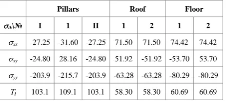
The maximal stresses of mining elements are observed in the neighbor of corners of chambers and theirs values presented in Tables 5, 6.
Table 5. Maximal values of stresses in pillars, Roof and Floor of chambers for Ω=0°
Pillars Roof Floor
σik\№ I 1 II 1 2 1 2
σxx -27.25 -31.60 -27.25 71.50 71.50 74.42 74.42
σxy -24.80 28.16 -24.80 51.92 -51.92 -53.70 53.70
σyy -203.9 -215.7 -203.9 -63.28 -63.28 -80.29 -80.29
[image:8.595.307.539.645.750.2]Table 6. Maximal values of stresses in pillars, Roof and Floor of chambers for Ω=30°
Pillars Roof Floor
σik\№ I 1 II 1 2 1 2
σxx -35,01 -37,14 -30,72 -63,26 -58,73 -66,37 -68,61
σxy 37,05 40,76 35,14 62,68 57,39 61,22 65,82
σyy -227,91 -244,53 -211,59 -76,66 -69,48 -83,08 -82,2
ΤI 115,64 124,26 108,31 67,67 61,58 65,48 70,95
It is seen (Table 5, 6), that for case Ω=30° the maximal stresses value exceed the stresses for Ω=30° from 5% to 18 %..
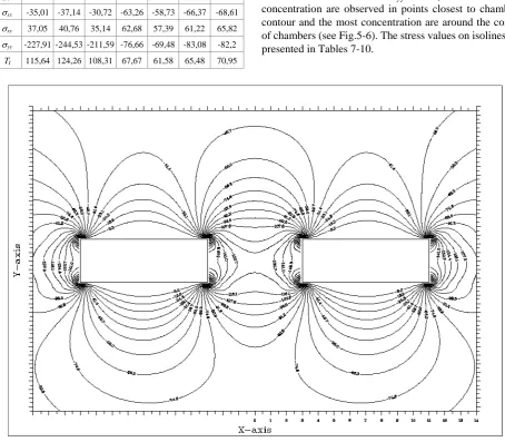
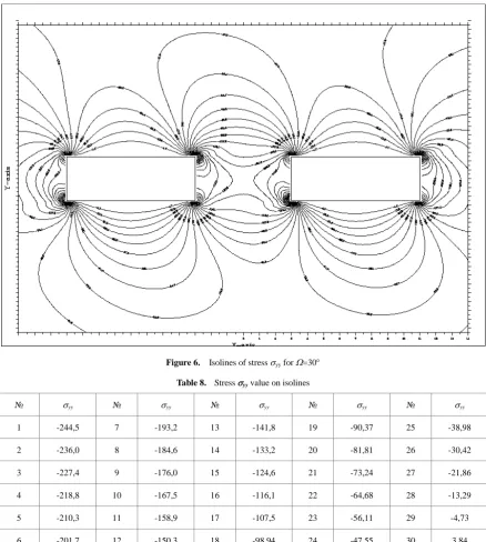
The isolines of stresses σyy and ΤI show that stress concentration are observed in points closest to chambers contour and the most concentration are around the corner of chambers (see Fig.5-6). The stress values on isolines are presented in Tables 7-10.
Figure 5. Isolines of stress σyy for Ω=0°
Table 7. Stress σyy value on isolines
№ σyy № σyy № σyy № σyy № σyy
1 -215.7 7 -171.1 13 -126.4 19 -81.8 25 -37.1
2 -208.3 8 -163.6 14 -118.9 20 -74.3 26 -29.7
3 -200.8 9 -156.2 15 -111.5 21 -66.9 27 -22.2
4 -193.4 10 -148.7 16 -104.1 22 -59.4 28 -14.8
5 -185.9 11 -141.3 17 -96.64 23 -52.0 29 -7.3
[image:9.595.68.523.126.523.2]Figure 6. Isolines of stress σyy for Ω=30°
Table 8. Stress σyy value on isolines
№ σyy № σyy № σyy № σyy № σyy
1 -244,5 7 -193,2 13 -141,8 19 -90,37 25 -38,98
2 -236,0 8 -184,6 14 -133,2 20 -81,81 26 -30,42
3 -227,4 9 -176,0 15 -124,6 21 -73,24 27 -21,86
4 -218,8 10 -167,5 16 -116,1 22 -64,68 28 -13,29
5 -210,3 11 -158,9 17 -107,5 23 -56,11 29 -4,73
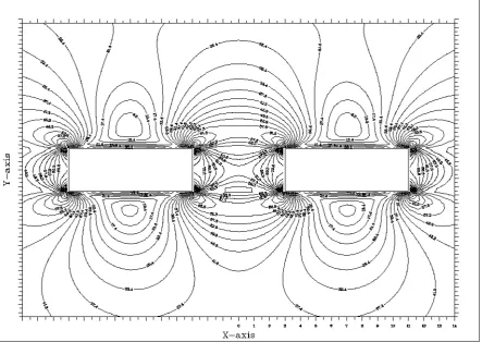
[image:10.595.78.517.76.565.2]Figure 7. Isolines of stress ΤI. for Ω=0°
Table 9. ΤΙ stress value on isolines
№ ΤΙ № ΤΙ № ΤΙ № ΤΙ № ΤΙ
1 5.47 7 26.9 13 48.36 19 69.80 25 91.3
2 9.04 8 30.5 14 51.93 20 73.38 26 94.8
3 12.6 9 34.1 15 55.51 21 76.9 27 98.4
4 16.2 10 37.6 16 59.08 22 80.5 28 101.9
5 19.9 11 41.21 17 62.65 23 84.1 29 105.5
[image:11.595.78.522.81.395.2] [image:11.595.76.521.427.585.2]Figure 8. Isolines of stress ΤI for Ω=30°
Table 10. ΤΙ stress value on isolines
№ ΤΙ № ΤΙ № ΤΙ № ΤΙ № ΤΙ
1 2,00 7 27,29 13 52,59 19 77,88 25 103,2
2 6,22 8 31,51 14 56,81 20 82,10 26 107,4
3 10,43 9 35,73 15 61,02 21 86,32 27 111,6
4 14,65 10 39,94 16 65,24 22 90,53 28 115,8
5 18,86 11 44,16 17 69,45 23 94,75 29 120,0
6 23,08 12 48,37 18 73,67 24 98,96 30 124,3
[image:12.595.75.525.427.570.2]Figure 9. Fragment of isolines of stress ΤI in interchamber pillar and corner regions of neighbor chambers for Ω=0°
[image:13.595.104.495.412.724.2]In case Ω=30° the Barrier pillar I is more loaded than Barrier pillar II, the Roof of chamber 1 more loaded than Roof of chamber 2 and Floor of chamber 2 more loaded than Floor of chamber 1 (Table 6). The stress field of right-upper corner of chamber 2 is cross symmetric to stress field of left-bottom left corner of chamber 2 and so on to stress field of right-bottom corner of chamber 1 and left-upper corner of chamber 2 (see Fig 10).
5. Conclusions
The fundamental solutions of the static problem for elastic plane with arbitrary anisotropic properties are obtained as the sum of residues of complex variable function. The assessment of fundamental solution and their derivatives are presented in closed form. In the distribution space are obtained the regular representations for the Somigliana formulas and the stress calculation formulas. These results are new and represent the subsequent development of the BEM method.
The test results performed for circular hole in anisotropic plane of rhombic system show a higher compliance for the boundary values of displacements and stresses calculated by proposed regular formulas. The results of analysis of the stress-strain state in the vicinity of rectangular mining chambers located in deep from day surface are presented in tables and pictures of isolines.
Acknowledgements
This research is financially supported by a grant from the Ministry of Science and Education of the Republic of Kazakhstan (Grant No. AP05135494).
REFERENCES
Tomlin, G.: Numerical analysis of continuum problems of [1]
zoned anisotropic media. Ph.D. thesis, Southampton University (1972).
Brebbia, C., Telles, J., Wrobel L.: Boundary element [2]
techniques: theory and applications in engineering. Springer-Verlag, Berlin (1984).
Vable M., Sikarskie D.: Stress analysis in plane orthotropic [3]
material by the boundary element method. Int. J. Solids Structures 24(1), 1–11 (1988).
Sun, X., Cen, Z.: Further improvement on fundamental [4]
solutions of plane problems for orthotropic materials. Acta Mechanica Solida Sinica 15 (2), 171–181 (2002).
Liu, Y., Huang, L. Sun, X., Cen, Z.: Boundary element [5]
analysis for elastic and elastoplastic problems of 2D orthotropic media with stress concentration. Acta Mechanica Sinica 21(5), 472-484 (2005).
Kolosova, E.: Fundamental solutions for anisotropic media [6]
and their applications (in Russian). Ph.D. thesis, South Federal University, Rostov-na-Donu (2007).
Hasebe, N., Sato, M.: Mixed boundary value problem for [7]
quasi-orthotropic elastic plane. Acta Mech 226(2), 527-545 (2015)
Ding, H ., Jiang, A. Chen, W.: Fundamental solutions for [8]
transversely isotropic magneto-electro-elastic media and boundary integral formulation. Science in China Series Е 46(6), 607–619 (2003).
Berger, J ., Martin, P., Mantič, V., Gray, L.: Fundamental [9]
solutions for steady-state heat transfer in an exponentially graded anisotropic material. Z. angew. Math. Phys. 56, 293–303 (2005).
Schiavone, P., Ru, C.: Integral equation methods in [10]
plane-strain elasticity with boundary reinforcement. Proc. R. Soc. Lond. A 454, 2223-2242 (1998).
Szeidl, G., Dudra, J.: Boundary integral equations for plane [11]
orthotropic bodies and exterior regions. Electronic Journal of Boundary Elements 8(2) 10-23 (2010).
Zozulya, V.: Regularization of the Divergent Integrals I. [12]
General consideration. Electronic Journal of Boundary Elements 4(2), 49-57 (2006).
Lekhnitskii, S.: Theory of elasticity of an anisotropic body. [13]
Mir Publishers, Moscow (1981).
Vladimirov V.: Equations of mathematical physics. (in [14]
Russian) Nauka, Moscow (1981).
Sh. A. Dildabayev, Sh., Zakir’yanova, G.: Fundamental [15]
solutions of the first and second boundary value problems of dynamics for an anisotropic elastic half-plane. (in Russian) Izvestya NAN Respuliki Kazakhstan ser. Fiz.-mat 5, 65-70 (1993).
Lachat JC, Watson JO. Effective numerical treatment of [16]
boundary integral equations – formulation for 3-dimensional elastostatics. International Journal for Numerical Methods in Engineering 1976; 10(5): 991-1005.
Clark S.: Handbook of physical constants. Geological [17]