R E S E A R C H
Open Access
Performance limit of AOA-based
localization using MIMO-OFDM channel state
information
Tanee Demeechai
*and Pratana Kukieattikool
Abstract
Wireless communication networks are increasingly based on the ubiquitous multiple-input multiple-output orthogonal frequency division multiplexing (MIMO-OFDM) modulation scheme. Their channel state information is generally obtained each time by a base station receiver as soon as a data packet is successfully received from a mobile device. As it has been shown recently that the MIMO-OFDM channel state information can be used for angle of arrival-based localization, this paper presents a theoretical investigation of the localization performance. The method of computing the Cramer-Rao lower bound, which represents the performance of a minimum variance unbiased estimator, is presented and then used for insightful investigation purposes by means of inspecting the viability of the system requirements and the design properties.
Keywords: Localization, Angle of arrival, MIMO-OFDM, Channel state information, Multipath propagation, Cramer-Rao lower bound
1 Introduction
Wireless localization is currently a research topic of pri-mary interest in the field of wireless communications due to providing a large variety of location-based services for increasingly ubiquitous smart mobile devices. For wireless localization, a method requiring hardware of just an exist-ing wireless network is of particular interest, because no extra hardware is required for both the infrastructure and the mobile devices (MDs). Unfortunately, although many studies have investigated wireless localization [1–5], it is not straightforward to apply their results without requir-ing dedicated hardware or affectrequir-ing the network protocol structure.
A few localization methods requiring hardware of just an existing wireless network have been proposed in the literature [6–9] and implemented commercially. Most of them [6–8] adopt fingerprint matching as the basic scheme of location determination. In this scheme, prior to the localization operation, algorithm parameters are determined by a training process. The parameters are
*Correspondence: [email protected]
National Electronics and Computer Technology Center, Phahonyothin Road, 12120 Pathum Thani, Thailand
determined in principle as a representation of the charac-teristics of the observation data associated with a number of MD reference locations. In the localization operation, the location is determined as a linear combination of the reference locations, based on the observation data and the trained parameters. One major drawback of this scheme is that the training process is usually a costly measurement process. In addition, because the radio wave propagation characteristics that characterize the observation data are sensitive to the environment, the training process will be required every time the environment of the localization region has changed.
We realize that the angle of arrival (AOA) estimation [10, 11] is an interesting study that can be applied for localization. Recently, it has been shown that multiple-input multiple-output (MIMO) orthogonal frequency division multiplexing (OFDM) channel state information (CSI) may be used as the observation data for localiza-tion based on AOA [9]. For localizalocaliza-tion based on AOA, it generally requires that direct radio paths between the MD and the base stations (BSs) are available sufficiently for triangulation. However, using MIMO-OFDM CSI as the observation data for localization based on AOA is of particular interest here, due to the following reasons.
AOA-based localization does not require a costly train-ing process. In addition, the MIMO-OFDM technique is currently the top air interface technology prevalently employed for very high-speed wireless networks.
The purpose of this paper is to investigate the perfor-mance characteristics of AOA-based localization methods that employ the MIMO-OFDM CSI as the observation data. This may be done by using the Cramer-Rao lower bound (CRLB), which is the variance of the estimation error of a minimum variance unbiased estimator (MVUE), as it has been successfully used to investigate theoreti-cal performance characteristics for a number of related estimation problems [12–14]. In this paper, a method of computing the CRLB in general for the AOA-based local-ization that uses MIMO-OFDM CSI as the observation data is presented. Numerical results are then obtained for a specific case detailing about the geometry and place-ment of the BS antenna arrays and the localization region. The results are discussed, respecting the impact of radio propagation characteristics and system infrastructures on the average system performance and providing funda-mental insights on the system requirements and design principles.
2 System and observation models
Channel frequency response (CFR) for a used OFDM sub-carrier is a necessary information for demodulation of data carried by that subcarrier. Conventionally, the trans-mitter needs to facilitate CFR estimation at the receiver by provision of pilot bits [15]. It is then reasonable to assume that once a receiver can successfully detect the data carried by the used OFDM subcarriers, it can also provide the CFR for the set of used OFDM subcarriers, i.e., the CSI, at no overhead. For localization, the CSI may be obtained, based on either uplink or downlink transmis-sion, for sending to a localization processor. In this paper, we are only interested in localization with processor resid-ing in the network infrastructure to avoid burdenresid-ing the generally resource-limited MDs. In this case, uplink CSI estimated by a BS receiver may be sent to the proces-sor at low cost via an existing non-radio connection. On the other hand, sending the downlink CSI estimated by a MD receiver to the processor inevitably requires some radio resource that can be costly. Reducing the cost of sending the downlink CSI to the processor may be done with a chunk-based scheme [16–18], where an average magnitude of CFR for a block of contiguous subcarriers is sent instead of the complex values of the CFR of all subcarriers within the block. However, AOA-based local-ization requires the CFR in complex form [9]. Therefore, strictly following [16–18] may not be appropriate for our problem. In this regard, we consider that a similar chunk-based scheme that sends an average complex CFR for the block instead of the average magnitude may be adopted
for AOA-based localization. This is because the average CFR obtained by this scheme is essentially same as that obtained by a conventional subcarrier-based scheme with the same total bandwidth but larger subcarrier spacing. However, this scheme therefore provides CFR with less details along the frequency axis. Accordingly, the proces-sor will perform worse on separating the direct path from reflection paths, leading eventually to lower performance. As using the uplink CSI for the localization proces-sor residing in the infrastructure is less cumbersome compared with using the downlink CSI, we assume that the location of a MD is determined by processing the CSI obtained by the MIMO-OFDM receivers of all BSs upon successful reception of a data packet from that MD. Assume that each BS employs an array of antennas, with the spacing between them on the order of half wave-length. Then, the CFR for theq-th BS respecting thek-th subcarrier andm-th antenna can be expressed by [9]
Hq,k,m= NP−1
n=0
gq,ne−j(2πtq,nk+φq,n,m)+wq,k,m, (1)
whereNPis the number of paths in the radio wave
prop-agation model, is the OFDM subcarrier spacing, gq,n
is the complex gain with magnitude representing the strength of the n-th path for the q-th BS, tq,n is the
propagation delay associated with then-th path between the MD antenna and the center of the antenna array of the q-th BS and subtracted by a constant delay specific to the q-th BS, φq,n,m, ∀m are the phase terms obeying
∀mφq,n,m = 0 and sharing a relationship that depends
on theq-th BS antenna array geometry and the AOA to the array from then-th path, andwq,k,mis the estimation
error that is assumed to behave as additive white Gaussian noise (AWGN). Assume that the terms in (1) have been sorted in ascending order of tq,n, i.e., tq,n1 ≤ tq,n2 if
n1 ≤ n2. In addition, it is required that direct path
from the MD antenna to the BS antenna array exists as the shortest path. Thus, it is the relationship betweenφq,0,m,
∀mthat contains the AOA-based location information of the MD.
synchronization, the receiver should be able to avoid inter-symbol interference (ISI) by beginning the demodulation of thel-th OFDM symbol att0withtd − tm ≤ t0 ≤ td.
Then, by virtue of the cyclic prefix, the orthogonality between the subcarriers is still preserved, and the direct path manifests itself to the synchronized demodulator as having delay oftq,0 = td − t0. Note that a good practice
of OFDM time synchronization is to havet0close totd.
Accordingly,tq,0 is usually a small non-negative number
compared with the guard interval length.
3 CRLB computation
The computation of CRLB can be based on the following theoretical assumptions. The number of antennas which are included in the array corresponds toMqfor theq-th
BS. Then, the observation data from theq-th BS may be expressed in a matrix form as
Hq,k =Sq,k+Wq,k, (2)
have used the following notations.
Aq= Note thataq(·)is a vector-valued function that depends
on theq-th BS antenna array geometry, andθq,ndenotes
the AOA to the array from then-th radio path. In addition, we have assumed that an AOA can be represented by a single number, and hence, two-dimensional localization is implied.
determined by the MD location given the geometry and placement of all the BS antenna arrays, we may define the row vector of independent parameters for the observation data as
u=x0 y0 v1 v2· · · vQ
, (7)
wherex0andy0represent the MD location in a Cartesian
coordinate system, and computation, we necessarily evaluate the derivative ofSq,k
with respect to each parameter, and we then obtain the following results.
LetSk denote the column vector of complete
observa-tion data for thek-th subcarrier:
Sk =
Then, based on [19], the Fisher information matrix for the parameter vectorucan be computed by
I=
where (·)Hdenotes the matrix conjugate and transpose,
andσ2is the variance ofw
q,k,m. Then, the CRLB for the
location error can be computed by
CRLB=I−11,1+I−12,2, (17) where [K]i,jdenotes the(i,j)element of matrixK.
4 Numerical results
4.1 Assumptions
4.1.1 Signal model
The following are assumed for the signal model. An antenna gain of 0 dB is assumed for the MD antenna as well as for each array element of a BS. The vari-ance of wq,k,m depends only on the system noise, i.e., E[|Hq,k,m − wq,k,m|2]/E[|wq,k,m|2] equals the average
signal-to-noise ratio per OFDM subcarrier. The noise figure of the OFDM receiver is 4 dB. The number of anten-nas in an antenna array is a constant, i.e.,Mq = M,∀q.
For the OFDM signal, the center frequency is 5.25 GHz, the subcarrier spacing follows that employed in [20], i.e., = 312.5 kHz, and the set of used subcar-rier indexes is {k| − K ≤ k ≤ K}, where
K is an integer controlling the bandwidth. We consider the bandwidth without accounting a guard band, i.e.,
B = (2K + 1) = (0.625K + 0.3125) MHz.
It should be noted that the total bandwidth BT
prac-tically allocated for the OFDM system is bigger than B. This is because guard bands are necessarily allocated to avoid interference from system of nearby spectrum. The guard bands may be implemented by having blocks of sub-carriers with zero amplitudes at both ends of the active spectrum. Hence, BT = (Nu + Nz), where Nu is
the number of used subcarriers 2K + 1, andNz is the
number of zero amplitude subcarriers. Then, we may note that while both the guard band and guard interval are necessarily allocated to deal with interference, they nec-essarily reduce the spectrum efficiency. Assume that the guard interval corresponds to cyclic prefix ofNcsample,
where the sampling rate is the nominal one for OFDM, i.e., 1/BT. Then, by the proper anticipation of guard band and
interval, the average rate of effectively carried information symbols is down-scaled byNu/(Nu + Nz + Nc)as noted
in [21].
4.1.2 Geometrical models
A linear array with half-wavelength spacing between ele-ments is assumed for each BS antenna array. Accordingly, the following geometrical reference model is applied. Cartesian coordinates (x0,y0) and (xq,yq) are used for
referring to the location of respectively the MD and the array center of theq-th BS. The relation between the two locations is represented as shown in Fig. 1 by a polar coor-dinate (rq,θq,0). The orientation of an antenna array is
represented by the normal looking direction of the array defined as follows. The normal looking direction is deter-mined by first setting the phase shifts of all the antenna elements to be zero and then determining the main radi-ation direction that is closest to the direction of arrival of the MD. We useγqto represent the normal looking
direc-tion for theq-th BS, as a counterclockwise angle relative to thex-axis. For example, if the placement line of theq-th BS antenna array is on thex-axis in Fig. 1,γqwill beπ/2.
Assuming rq is much greater than the spacing between
Fig. 1Illustration of geometrical reference model. Illustration of geometrical reference model of (x0,y0), (xq,yq), (rq,θq,0), andγq
the antenna array elements, thenφq,n,m,∀(q,n,m)can be
approximated by
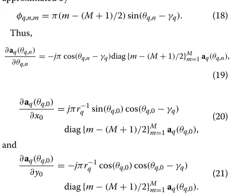
φq,n,m=π(m−(M+1)/2)sin(θq,n−γq). (18)
Thus,
∂aq(θq,n)
∂θq,n = −
jπcos(θq,n−γq)diag{m−(M+1)/2}Mm=1aq(θq,n),
(19)
∂aq(θq,0) ∂x0 =
jπrq−1sin(θq,0)cos(θq,0−γq)
diag{m−(M+1)/2}Mm=1aq(θq,0),
(20)
and
∂aq(θq,0) ∂y0 = −
jπr−q1cos(θq,0)cos(θq,0−γq)
diag{m−(M+1)/2}Mm=1aq(θq,0).
(21)
The performance results will be obtained by averaging the computed CRLBs over various values of the parameter vectoru. Figure 2 shows the geometrical assumptions, on which the variation ofuis based. It shows that the region of interest for localization is a square with area of 400 m2,
there is a BS located at each corner, and the normal look-ing directions of the four arrays are pointed towards the region center.
4.1.3 Multipath propagation model
Fig. 2Illustration of geometrical simulation assumptions. The 400-m2 region of interest for localization and the normal looking directions of the antenna arrays of four BSs located at the corners
The direct path The direct path parameters for theq-th
BS consist of onlygq,0andωq,0, becauseθq,0can be
deter-mined formx0andy0. In this paper,∠gq,0is drawn from
a uniform distribution over [ 0, 2π), and|gq,0|is obtained,
based on the free-space path loss model. Assume the vari-ance ofwq,k,misσ2= 1. Also, recall that the gain of each
antenna is 0 dB. Thus,
|gq,0|2=Pt
c
4πfcrq
2
/(κTeB), (22)
wherePtis the MD transmitted power,cis the light speed, fc = 5.25E+9 Hz as assumed,κ is the Boltzmann
con-stant, andTe is the effective noise temperature of the BS
receiver. For the value ofωq,0, we settq,0=0, based on the
discussion in Section 2.
The reflection paths In this paper,∠gq,nandθq,n,∀n>0
are independently drawn from a uniform distribution over [ 0, 2π). In addition,|gq,n|andωq,n,n>0 are set to obey
|gq,n−1|2
|gq,n|2 =ρ
, (23)
and
tq,n−tq,n−1=δ, (24)
where ρ reflects a constant power-decay condition, and
δ−1 reflects the multipath density. The magnitude of a
reflection path is not modeled to have a random charac-teristic, as it is treated as a controlled variable of the study. However, as the reflection paths are delayed relative to the direct path and their complex amplitudes have identical and independent random phases, the frequency response over the frequency band of the signal has a random
frequency-selective fading characteristic. In this regard, we may note from (1) that the CFR for a specific subcarrier is a summation of independent complex zero mean circu-larly symmetric random variables. Hence, for largeNP ,
the frequency response over a subcarrier could exhibit fre-quency flat-fading characteristics with Rayleigh or Rician distribution, the common characteristics in practical radio propagation environments [22]. The Rayleigh distribution could occur when|gq,0|2
NP−1
n=1 |gq,n|2, which is
pos-sible withρ ≈ 1. This is because whenρ = 1, we have |gq,n| = |gq,0|for alln > 0 and accordingly the RicianK
factor [22] is 1/(NP−1)≈0. On the other hand, the Rician
distribution could occur when|gq,0|2 Nn=P−11|gq,n|2,
which is possible withρ1.
4.2 Discussion
The mean square error (MSE) performance results pre-sented here are obtained by averaging the computed CRLBs over various values of the parameter vectoru. In this regard, the MD is uniformly and randomly located in the 400-m2region, except the locations that are close to the center of an antenna array by less than 1 m. The perfor-mance will be presented forPt= −20 dBm, respecting the
infrastructure conditions (BandM) and the radio prop-agation characteristics (ρ, δ, andNP). The performance
respectingPt is not presented, because it is obvious that
the MSE-versus-Ptcurve in this case is a line with a slope
of−10 dB/decade. Note also that a study of the perfor-mance respecting geometry may be useful in determining the positions of BS antenna arrays [23]. Such study is beyond the scope of our work, and we believe it merits further investigation.
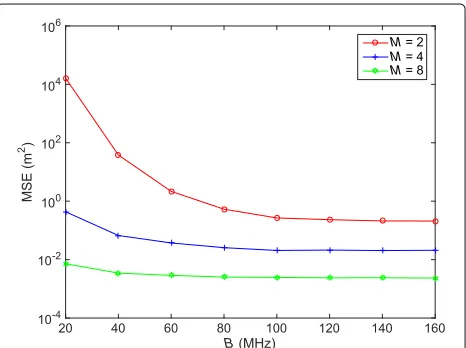
Figures 3 and 4 show the MSE performance in relation to B and M, for δ = 10 ns, ρ = 0 dB, and NP = 5.
Note that changingMaffects the quantity of observation
20 40 60 80 100 120 140 160
B (MHz) 10-4
10-2 100 102 104 106
MSE (m
2)
M = 2 M = 4 M = 8
2 4 6 8 10 12 14 16
M
10-4 10-2 100 102 104 106
MSE (m
2 )
B = 20 MHz
B = 40 MHz
B = 80 MHz
Fig. 4Numerical result 2. MSE versusMwithBas a parameter, for δ=10 ns,ρ=0 dB, andNP=5
data and accordingly the number of rows ofEkthat equals QM. Also, changingBaffects the quantity of observation data and accordingly the number of summands in (16) that equals 2K+1. In addition, by changingB, we must recom-putegq,n,∀(q,n), according to (22) and (23), for use in the
construction of newEk. Figure 3 shows that the MSE may
be reduced by increasingB, but there is a limit where the MSE cannot be reduced further. According to the figure, that limit is found to be reachable at smallerBfor largerM. That limit is also found to depend onM, as the limits for
M=2, 4, and 8 are respectively about 0.2094, 0.0201, and 0.0023 m2. Figure 4 shows that the MSE may be reduced by increasing M. However, as M becomes larger, the MSE always decreases while the importance ofBbecomes lesser, as the MSE limit discussed above is being reached. Hence, the above observations may be summarized as fol-lows. The MSE performance can be generally improved by increasing eitherBorM, but increasingBcan only reduce the MSE to a limit depending onM. IncreasingMalone can push the MSE to the limit, which is also smaller asM
increases. In addition, with a largerM, a smallerBwould be required for the MSE to approach the limit.
Figure 5 shows the MSE performance in relation toNP
and M, for B = 40 MHz, δ = 10 ns, andρ = 0 dB, which includes the free-space results (NP =1). Note that
changingNPaffects the number of parameters for
estima-tion and accordingly the number of columns ofEk that
equals (4NP −1)Q+ 2. Interestingly, it should be first
noted that the free-space results in Fig. 5 and the MSE limits in Fig. 3 are same. This suggests that the MSE limit previously discussed corresponds to the performance vir-tually obtained from free-space channel. Hence, in this paper, we will refer to the free-space channel result as the free-space limit. This limiting characteristic of the MSE is consistent with the following principles. First, note from
1 2 3 4 5 6 7 8 9 10
Np
10-4 10-2 100 102 104 106
MSE (m
2 )
M = 2
M = 4
M = 8
Fig. 5Numerical result 3. MSE versusNPwithMas a parameter, for B=40 MHz,δ=10 ns, andρ=0 dB
(1) that the contribution of a particular path is a com-plex sinusoidal function ofkwith a particular frequency depending on the path delay. In this regard, we should note that direct-path AOA estimation basically requires separating the direct-path contribution from reflection-path contributions, where largeBis of great help. This is because of that the key difference between the paths is the sinusoidal frequency and that a less ambiguous result on such frequency determination basically requires observ-ing the CFR over a larger range ofk. Then, onceBis large enough for perfect path separation, further increasingB
while retaining the total transmitted power as assumed here is not seen to further improve the localization perfor-mance. This indicates that AOA estimation performance for a perfectly separated path depends on the total trans-mitted signal power, regardless of the signal bandwidth. Hence, increasingBby more spreading of the fixed trans-mitted power over the spectrum can only help the MVUE separate the multipaths, which eventually pushes the per-formance to approach the free-space limit. Figure 5 also shows that the logarithm of the MSE rises almost linearly withNPforM =2, while for otherM, the MSE remains
almost constant even ifNP is close to 10. The results for NP = 5 in Fig. 5 are consistent with the results of the
same case, i.e., B = 40 MHz, in Fig. 3. The results of the mentioned case from both figures consistently indi-cate that the MSE is far from the free-space limit for
M = 2, while for other M, the MSE is already close to the free-space limit. Hence, if the MSE is already close to the free-space limit due to an appropriate provision ofBandMto deal with the multipath environment, the MVUE will be robust against variation ofNP. Otherwise,
the corresponding MSE will rise exponentially withNP.
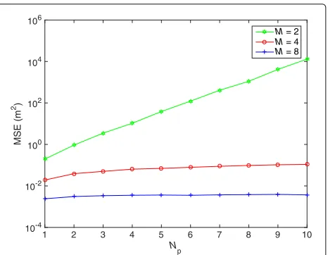
Figure 6 shows the MSE performance in relation to
1 2 3 4 5 6 7 8 9 10
Np
10-1 100 101 102 103 104 105
MSE (m
2)
B = 40 MHz
B = 80 MHz
B = 160 MHz
Fig. 6Numerical result 4. MSE versusNPwithBas a parameter, for M=2,δ=10 ns, andρ=0 dB
The figure provides same observations as previously dis-cussed, regarding the characteristics of MSE againstNP
and impact of increasingBon the MSE performance for multipath environments. Interestingly, it also shows that the free-space results do not depend onB. Theoretically, this may be justified by the following considerations. For
NP = 1, (1) becomes Hq,k,m = gq,0e−j(ωq,0k+φq,0,m) + wq,k,m. The AOA-based localization basically relies on the
estimation ofφq,0,m,∀(q,m), in which the AOA
informa-tion is contained. As a result of [24], we note that the CRLB of φq,0,m based on the(2K +1)sample
observa-tion ofHq,k,mis inversely proportional to|gq,0|2(2K+1)
for large K. Recall that B = (2K + 1), and |gq,0|2B is proportional to Pt according to (22).
There-fore, |gq,0|2(2K + 1) is also proportional to Pt. In
addi-tion, the CRLB of φq,0,m depends on Pt, instead of B.
Note also that by first-order approximation, the associ-ation between a small error of φq,0,m and the resulting
localization error is approximately linear. Therefore, the free-space localization CRLB results also depend on Pt,
instead ofB.
Finally, regarding comparison between the impacts ofB
andMon the MSE performance, we note from Figs. 3, 4, 5 and 6 that doublingMgives greater performance benefit than doublingBfor all cases observable from the figures. This should come from the following principles of AOA-based localization using (1). IncreasingBwhile maintain-ingPtonly helps the MVUE separate the multipaths. On
the other hand, increasing M not only provides more observation data that help multipath separation but also improves AOA sensitivity and therefore the free-space limit.
Figure 7 shows the MSE performance in relation to δ and M, for B = 80 MHz, ρ = 0 dB, and NP = 10,
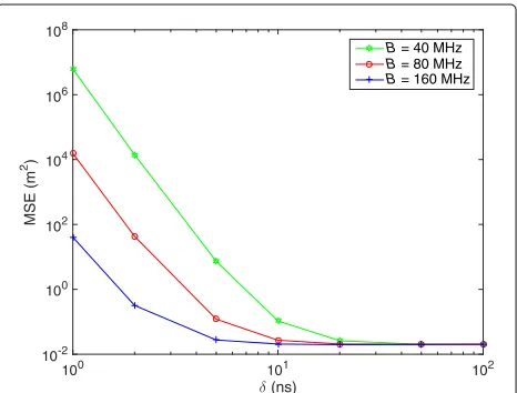
while Fig. 8 shows the MSE performance in relation toδ
100 101 102
(ns) 10-4
10-2 100 102 104 106
MSE (m
2)
M = 4
M = 8
M = 16
Fig. 7Numerical result 5. MSE versusδwithMas a parameter, for
B=80 MHz,ρ=0 dB, andNP=10
andB, forM = 4,ρ = 0 dB, andNP = 10. Note that
changingδdoes not affect either the size ofEkor the num-ber of summands in (16), because it does not affect either quantity of observation data or the number of parameters for estimation. By changingδ , we only recompute ωq,n, n > 0,∀q to obey (24) for use in the construction of newEk. Below are the reported various observations from
the figures. The multipath density has a profound impact on the MSE performance, as the performance tends to get severely worse than the free-space limit whenδ is lower than a certain boundary value that can be reduced by increasingBorM. For example, it can be seen from Fig. 7 that forM = 4, the MSE starts to get worse than the free-space limit when theδ is decreasing below a value between 5 and 10 ns, while for a largerM, such character-istic occurs at a smallerδ. It can be also seen from Fig. 8
100 101 102
(ns) 10-2
100 102 104 106 108
MSE (m
2)
B = 40 MHz
B = 80 MHz
B = 160 MHz
Fig. 8Numerical result 6. MSE versusδwithBas a parameter, for
that forB = 40 MHz, the MSE starts to get worse than the free-space limit when theδis decreasing below a value between 10 and 20 ns, while for a largerB, such character-istic occurs at a smallerδ. It may be also noted from Fig. 7 that in addition to reducing the boundary value, provision for a largerMalso reduces the rate of deterioration when theδdecreases below beyond the boundary value. Again, regarding comparison between the impacts ofBandMon the MSE performance, we see that increasingMprovides greater performance benefit.
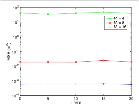
Figure 9 shows the MSE performance in relation toρ andM, forB = 80 MHz,δ = 2 ns, andNP = 10. Note
that changingρ does not affect either the size ofEk or
the number of summands in (16). By changingρ, we only recomputegq,n,n > 0,∀qto obey (23) for use in the
con-struction of newEk. The figure shows that all curves are
essentially flat, and therefore, the MSE seems to be inde-pendent ofρ. Comparing the MSE results in Fig. 9 and the free-space limits observable from Fig. 7, we see that the MSE at δ = 2 ns is farthest to the free-space limit when M = 4, while it is nearest when M = 16. The flat characteristic of the curves in Fig. 9 exists, no matter how far from the free-space limit the MSE is. This may sound surprising, because the channel at ρ = 20 dB is very much alike a free-space channel, and for this con-dition, one can easily design an algorithm that performs very close to the free-space limit. An algorithm that simply treats the channel as a free-space channel should be able to achieve such performance, because that insignificant model mismatch should only cause insignificant bias to the estimation result. This also means that when the mod-eled reflection paths are weak, the MVUE could perform surprisingly as poor as the case where the paths are strong. Such behavior of the MVUE, which embraces all modeled paths into its idealized unbiased estimation task, will be
0 5 10 15 20
(dB) 10-4
10-3 10-2 10-1 100 101 102
MSE (m
2 )
M = 4
M = 8
M = 16
Fig. 9Numerical result 7. MSE versusρwithMas a parameter, for
B=80 MHz,δ=2 ns, andNP=10
mathematically justified soon in this section. Hence, we suggest that reflection paths with insignificant amplitude should not be included explicitly in the channel model. This is to maintain that the CRLB may be also meaningful in a study of biased estimation algorithms.
We may claim more strictly from the results in Fig. 9 that the localization performance of the MVUE is inde-pendent of the strength of a reflection path. This can be mathematically justified by the following considerations. Note that the gain of a particular reflection path appears as a constant factor consistently for all non-zero elements along only two columns ofEk. For a specificgq,n,n > 0,
such two columns correspond to respectively the (n+1)-th column ofD()q,k and then-th column ofD()q,k. The indexes of them within Ek are always greater than two, because they all belong toD(q∗,k) in (15). Therefore, by scaling the value of thegq,nwith a real factor,Ekcan be recomputed
accordingly by post-multiplying itself with a real constant diagonal matrix, where all diagonal elements are equal to one except the elements associated with the two indexes. The inverse of the Fisher information matrix can then be recomputed by pre- and post-multiplying itself with the inverse of that diagonal matrix. Such operation will not affect the localization performance of the MVUE com-puted by (17), because the two indexes are always greater than two.
We have been realizing from the results of Figs. 7 and 8 that the multipath density reflected byδis crucial to the effectiveness of the infrastructure reflected byBandM. However, we consider that care may be only required for the second path that has delay closest to the direct path, because it contributes most to the difficulty of separating the direct path from other paths. Thus, it may be more interesting to investigate the case of channels where the path delay rule in (24) is replaced by
tq,n−tq,n−1=
δ0, ifn=1
δ1, otherwise. (25) Figure 10 shows the MSE performance in relation to
δ1and B, forM = 4, ρ = 0 dB, NP = 10, δ0 = 10
1 2 3 4 5 6 7 8 9 10
1 (ns)
10-2 10-1 100 101 102 103
MSE (m
2)
B = 40 MHz
B = 80 MHz
B = 160 MHz
Fig. 10Numerical result 8. MSE versusδ1withBas a parameter, for M=4,ρ=0 dB,NP=10, andδ0=10 ns
MD and the BS. For such a position, we may further note that everyone around the BS is most cumbersome. This is because the corresponding reflection path AOA can be considerably different from the direct-path AOA, and then, the reflection path needs to be modeled explicitly as having such different AOA but similar delay to that of the direct path. On the other hand, for such a scatterer position rather than those around the BS, the correspond-ing reflection path AOA cannot be considerably different from the direct-path AOA. Accordingly, by neglecting the seen insignificant difference on both the delay and AOA, the reflection path can be approximately modeled by merging itself with the direct path based on only com-plex path-amplitude addition. Therefore, it is important to avoid the most cumbersome scatterers by ensuring that the BS antenna arrays are carefully placed not close to any significant reflective materials, and in some cases, using radio-absorptive materials may be helpful.
5 Conclusions
We studied the problem of AOA-based localization using MIMO-OFDM channel state information as observation data. In particular, we derived a method to compute the CRLB which is a fundamental limit on the localiza-tion MSE and applied it to obtain fundamental insights into the problem. We found that the CRLB is indepen-dent of the strength of a reflection path. Therefore, we suggested that reflection paths with insignificant ampli-tude should not be included explicitly in the channel model. Provided that the mobile device-transmitted sig-nal power is fixed, the following may be concluded from our investigation. The MSE localization performance can be improved by increasing the transmitted signal band-width B alone. However, there is a limit where further
increasing B cannot further improve the performance. The limit is found to equal the performance virtually obtained from the free-space radio propagation assump-tion. The performance can be considerably improved also by increasing the base station antenna array sizeMalone, as, whenMincreases, not only does the free-space limit decrease but also the MSE gets closer to the decreas-ing limit. In particular, scaldecreas-ing M always has greater impact on the MSE than scaling B. Provided that the MSE is close to the free-space limit, the optimum unbi-ased estimator will be robust to variation on the number of multipaths NP. Otherwise, the MSE will rise
expo-nentially withNP. The multipath density that is inversely
proportional toδhas a profound impact on the MSE per-formance, as the performance tends to get severely worse than the free-space limit when the density is higher than a value proportional to B andM. Finally, when signifi-cant reflection paths with AOAs very different from that of the direct path have similar delays to that of the direct path, the localization performance could be severely degraded.
Acknowledgements
The authors would like to thank the anonymous reviewers for their constructive comments, which helped a lot to improve the presentation of this paper.
Funding Not applicable.
Authors’ contributions
Both authors contributed to the searching of the literature. TD contributed to theoretical analysis. Both authors contributed to the design and
implementation of computer simulation experiments and interpretation of the results. Both authors have read and approved the final manuscript.
Competing interests
The authors declare that they have no competing interests.
Publisher’s Note
Springer Nature remains neutral with regard to jurisdictional claims in published maps and institutional affiliations.
Received: 9 January 2017 Accepted: 4 August 2017
References
1. H Liu, H Darabi, P Banerjee, J Liu, Survey of wireless indoor positioning techniques and systems. IEEE Trans. Syst. Man Cybern. Part C Appl. Rev. 37(6), 1067–1080 (2007)
2. Z Farid, R Nordin, M Ismail, Recent advances in wireless indoor localization techniques and system. J. Comput. Netw. Commun.2013(185138), 1–12 (2013)
3. K Yu, I Sharp, YJ Guo,Ground-based wireless positioning, 1st edn. (Wiley, West Sussex, 2009)
4. Y Zhao, K Liu, Y Ma, Z Li, An improved k-NN algorithm for localization in multipath environments. EURASIP J. Wirel. Commun. Netw.2014(208), 1–10 (2014)
5. MB Zeytinci, V Sari, FK Harmanci, E Anarim, M Akar, Location estimation using RSS measurements with unknown path loss exponents. EURASIP J. Wirel. Commun. Netw.2013(178), 1–14 (2013)
7. M Youssef, A Agrawala, inProceedings of the 3rd International Conference on Mobile Systems, Applications, and Services. The Horus WLAN Location Determination System (Association for Computing Machinery (ACM), New York, 2005), pp. 205–218
8. K Wu, J Xiao, Y Yi, D Chen, X Luo, LM Ni, CSI-based indoor localization. IEEE Trans. Parallel Distrib. Syst.24(7), 1300–1309 (2013)
9. T Demeechai, P Kukieattikool, T Ngo, T-G Chang, Localization based on standard wireless lan infrastructure using mimo-ofdm channel state information. EURASIP J. Wirel. Commun. Netw.2016(146), 1–16 (2016) 10. NB Rejeb, I Bousnina, MBB Salah, A Samet, Joint mean angle of arrival,
angular and Doppler spreads estimation in macrocell environments. EURASIP J. Adv. Signal Process.2014(133), 1–10 (2014)
11. SO Al-Jazzar, A Muchkaev, A Al-Nimrat, M Smadi, Low complexity and high accuracy angle of arrival estimation using eigenvalue decomposition with extension to 2D AOA and power estimation. EURASIP J. Wirel. Commun. Netw.2011(123), 1–13 (2011)
12. Y Shen, MZ Win, Fundamental limits of wideband localization: Part I: a general framework. IEEE Trans. Inf. Theory.56(10), 4956–4980 (2010) 13. H Godrich, AM Haimovich, RS Blum, Target localization accuracy gain in
mimo radar-based systems. IEEE Trans. Inf. Theory.56(6), 2783–2803 (2010)
14. K Witrisal, E Leitinger, S Hinteregger, P Meissner, Bandwidth scaling and diversity gain for ranging and positioning in dense multipath channels. IEEE Wirel. Commun. Lett.5(4), 396–399 (2016)
15. H Minn, N Al-Dhahir, Optimal training signals for MIMO OFDM channel estimation. IEEE Trans. Wirel. Commun.5(5), 1158–1168 (2006)
16. H Zhu, J Wang, Chunk-based resource allocation in OFDMA systems—part I: chunk allocation. IEEE Trans. Commun.57(9), 2734–2744 (2009) 17. H Zhu, J Wang, Chunk-based resource allocation in OFDMA
systems—part II: Joint chunk, power and bit allocation. IEEE Trans. Commun.60(2), 499–509 (2012)
18. H Zhu, Radio resource allocation for OFDMA systems in high speed environments. IEEE J. Sel. Areas Commun.30(4), 748–759 (2012) 19. SM Kay,Fundamentals of statistical signal processing: estimation theory.
(Prentice Hall, New Jersey, 1993), p. 47
20. IEEE Std 802.11ac - 2013, IEEE Standard for Information
Technology-Telecommunications and information exchange between systems ˝Ulocal and metropolitan area networks-specific requirements, Part 11: wireless LAN medium access control (MAC) and physical layer (PHY) specifications, Amendment 4: enhancements for very high throughput for operation in bands below 6 GHz. (The Institute of Electrical and Electronics Engineers, Inc., New York, NY, USA, 2013) 21. SK Chronopoulos, C Votis, V Raptis, G Tatsis, P Kostarakis, inAIP Conference
Proceedings 1203. in depth analysis of noise effects in orthogonal frequency division multiplexing systems, utilising a large number of subcarriers (American Institute of Physics (AIP), New York, 2010), pp. 967–972
22. SK Chronopoulos, V Christofilakis, G Tatsis, P Kostarakis, Performance of turbo coded OFDM under the presence of various noise types. Wirel. Pers. Commun.87(4), 1319–1336 (2016)
23. W Shi, X Qi, J Li, S Yan, L Chen, Y Yu, X Feng, Simple solution to the optimal deployment of cooperative nodes in two-dimensional TOA-based and AOA-based localization system. EURASIP J. Wirel. Commun. Netw.2017(79), 1–16 (2017)
24. DC Rife, RR Boorstyn, Single-tone parameter estimation from