1
Supplementary Materials
Transitions from single- to multi-locus processes during speciation
Schilling MP, Mullen SP, Kronforst M, Safran RJ, Nosil P, Feder JL, Gompert Z, and Flaxman SM
2018
Table S1: Summary statistics for the 300 included simulation runs.
set A B C D E F
s 0.005 0.01 0.02 0.005 0.01 0.02
m 0.01 0.01 0.01 0.1 0.1 0.1
nRuns 50 50 50 50 50 50
mean number of variable loci 2386.02 1077.2 554.48 197.02 1202.46 626.3 sd number of variable loci 56.67 36.94 23.93 13.59 32.47 22.02 mean total generations elapsed 619540 155160 39979.68 1500000 333960 63230 sd total generations elapsed 24938.46 8524.54 2970.84 0 32459.68 5090.22
RI reached 1 1 1 0 1 1
mean total mutations introd. 6195409 1551609 399805.8 15000000 3339609 632309 sd total mutations introd. 249384.6 85245.38 29708.39 0 324596.8 50902.17
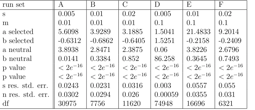
Table S2: Summary for nonlinear least squares fit of Barton’s coupling coefficient (θ) and average allele frequency differences between demes for selected and neutral loci.
run set A B C D E F
s 0.005 0.01 0.02 0.005 0.01 0.02
m 0.01 0.01 0.01 0.1 0.1 0.1
a selected 5.6098 3.9289 3.1885 1.5041 21.4833 9.2014 b selected -0.6312 -0.6862 -0.6405 1.5251 -0.2158 -0.2409 a neutral 3.8938 2.8471 2.3875 0.06 3.8226 2.6796 b neutral 0.0141 0.3384 0.852 86.258 0.3645 0.7493 p value <2e−16 <2e−16 <2e−16 <2e−16 <2e−16 <2e−16
p value <2e−16 <2e−16 <2e−16 <2e−16 <2e−16 <2e−16 s res. std. err. 0.0243 0.0231 0.0316 0.003 0.0557 0.055 n res. std. err. 0.0302 0.0294 0.026 0.00059 0.0355 0.031
2
Table S3: Summary for nonlinear least squares fit of average LD for selected and neutral loci. Run D did not yield intelligible results and was excluded here.
run set A B C D E F
s 0.05 0.01 0.02 0.005 0.01 0.02
m 0.01 0.01 0.01 0.1 0.1 0.1
z selected 0.962 0.935 0.905 – 0.948 0.918
a selected 0.0614 0.1835 0.076 – 0.213 0.273
b selected 81.12 16.927 28.774 – 161.3 37.05
z neutral 0.729 0.463 0.1892 – 0.508 0.245
a neutral 0.0147 0.0361 0.0167 – 0.0314 0.0406
b neutral 231.6 80.5 166 – 234.6 90.06
p value <2e−16 <2e−16 <2e−16 – <2e−16 <2e−16
p value <2e−16 <2e−16 <2e−16 – <2e−16 <2e−16
s res. std. err. 0.0208 0.03326 0.0428 – 0.035 0.039 n res. std. err. 0.0312 0.016 0.0063 – 0.015 0.0095
df 664 167 289 – 401 151
Table S4: Numbers of scffolds and variants for each invludedHeliconius chromosome. Chromosome no. scaffolds no. variants
2 1 449,499
7 1 667,749
10 1 850,334
18 3 771,594
21 (Z) 1 523,014
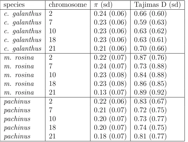
Table S5: Population genetic statistics for Heliconius species per chromosome. species chromosome π (sd) Tajimas D (sd)
c. galanthus 2 0.24 (0.06) 0.66 (0.60)
c. galanthus 7 0.23 (0.06) 0.59 (0.63)
c. galanthus 10 0.23 (0.06) 0.63 (0.62)
c. galanthus 18 0.23 (0.06) 0.63 (0.61)
c. galanthus 21 0.21 (0.06) 0.70 (0.66)
m. rosina 2 0.22 (0.07) 0.87 (0.76)
m. rosina 7 0.24 (0.07) 0.73 (0.88)
m. rosina 10 0.23 (0.08) 0.84 (0.88)
m. rosina 18 0.23 (0.08) 0.86 (0.85)
m. rosina 21 0.13 (0.07) 0.89 (0.92)
pachinus 2 0.22 (0.06) 0.83 (0.67)
pachinus 7 0.21 (0.07) 0.72 (0.75)
pachinus 10 0.20 (0.07) 0.73 (0.77)
pachinus 18 0.20 (0.07) 0.74 (0.75)
3 Table S6: Population genetic statistics for Heliconius species pairs per chromosome
species pair chromosome FST (sd) dxy (sd) no. outliers
(AFDs & FST,
resp.)
99% quant. AFDs
99% quant. FST
c. galanthus - m. rosina 2 0.23 (0.25) 0.37 (0.09) 4495 0.9484 0.9513
c. galanthus - m. rosina 7 0.22 (0.25) 0.37 (0.10) 6677 0.9274 0.9499
c. galanthus - m. rosina 10 0.25 (0.26) 0.38 (0.09) 8503 0.9495 0.95
c. galanthus - m. rosina 18 0.25 (0.27) 0.38 (0.10) 7716 0.9967 0.9912
c. galanthus - m. rosina 21 0.39 (0.33) 0.46 (0.11) 5230 0.9963 0.9963
pachinus - m. rosina 2 0.27 (0.27) 0.38 (0.09) 4495 0.9848 0.9907
pachinus - m. rosina 7 0.27 (0.27) 0.39 (0.10) 6677 0.9573 0.9677
pachinus - m. rosina 10 0.30 (0.28) 0.40 (0.10) 8503 0.9912 0.9933
pachinus - m. rosina 18 0.29 (0.28) 0.40 (0.11) 7716 0.9967 0.9981
pachinus - m. rosina 21 0.44 (0.35) 0.48 (0.12) 5230 0.9963 0.998
c. galanthus - pachinus 2 0.09 (0.13) 0.26 (0.06) 4495 0.4152 0.4399
c. galanthus - pachinus 7 0.08 (0.13) 0.25 (0.06) 6677 0.3999 0.4112
c. galanthus - pachinus 10 0.09 (0.14) 0.24 (0.06) 8503 0.4233 0.4188
c. galanthus - pachinus 18 0.09 (0.13) 0.24 (0.06) 7716 0.4019 0.422
4 Figure S1: Venn diagrams to illustrate the overlap of outliers for A) AFDs and B) FST and all species pairs and chromosomes.
Percentage of overlap is shown for respective pairs of taxa. C) Percentage of overlap between AFD and FST species pairs and
5
6
Figure S3: Density curves of coupling coefficients for loci at different types of sites on chromosome 10, determined by outliers of AFDs. Log r2 values are shown between
7
Figure S4: Density curves of coupling coefficients for loci at different types of sites on chromosome 18, determined by outliers of AFDs. Log r2 values are shown between
8
Figure S5: Density curves of coupling coefficients for loci at different types of sites on chromosome 2 and respective sites on all other chromosomes, determined by outliers of AFDs. Log r2 values are shown between selected loci, between neutral loci and between
selected and neutral loci for species pairs of H. cydno galanthus and H. melpomene rosina
9
Figure S6: Density curves of coupling coefficients for loci at different types of sites on chromosome 7 and respective sites on all other chromosomes, determined by outliers of AFDs. Log r2 values are shown between selected loci, between neutral loci and between
selected and neutral loci for species pairs of H. cydno galanthus and H. melpomene rosina
10
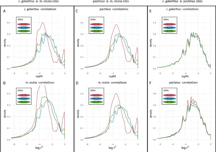
Figure S7: Density curves of coupling coefficients for loci at different types of sites on chromosome 10 and respective sites on all other chromosomes, determined by outliers of AFDs. Log r2 values are shown between selected loci, between neutral loci and
between selected and neutral loci for species pairs of H. cydno galanthus and H. melpomene rosina (A & B), H. pachinus and H. melpomene rosina (C & D), and H. cydno galanthus
11
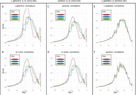
Figure S8: Density curves of coupling coefficients for loci at different types of sites on chromosome 18 and respective sites on all other chromosomes, determined by outliers of AFDs. Log r2 values are shown between selected loci, between neutral loci and
between selected and neutral loci for species pairs of H. cydno galanthus and H. melpomene rosina (A & B), H. pachinus and H. melpomene rosina (C & D), and H. cydno galanthus
12
Figure S9: Density curves of coupling coefficients for loci at different types of sites on chromosome 21 and respective sites on all other chromosomes, determined by outliers of AFDs. Log r2 values are shown between selected loci, between neutral loci and
between selected and neutral loci for species pairs of H. cydno galanthus and H. melpomene rosina (A & B), H. pachinus and H. melpomene rosina (C & D), and H. cydno galanthus
13
Figure S10: Density curves of coupling coefficients for loci at different types of sites on chromosome 2, determined by FST outliers. Log r2 values are shown between selected
14
Figure S11: Density curves of coupling coefficients for loci at different types of sites on chromosome 7, determined by FST outliers. Log r2 values are shown between selected
15
Figure S12: Density curves of coupling coefficients for loci at different types of sites on chromosome 10, determined by FST outliers. Log r2 values are shown between selected
16
Figure S13: Density curves of coupling coefficients for loci at different types of sites on chromosome 18, determined by FST outliers. Log r2 values are shown between selected
17
Figure S14: Density curves of coupling coefficients for loci at different types of sites on chromosome 21, determined by FST outliers. Log r2 values are shown between selected
18
Figure S15: Density curves of coupling coefficients for loci at different types of sites on chromosome 2 and respective sites on all other chromosomes, determined by FST
outliers. Log r2 values are shown between selected loci, between neutral loci and between
selected and neutral loci for species pairs of H. cydno galanthus and H. melpomene rosina
19
Figure S16: Density curves of coupling coefficients for loci at different types of sites on chromosome 7 and respective sites on all other chromosomes, determined by FST
outliers. Log r2 values are shown between selected loci, between neutral loci and between
selected and neutral loci for species pairs of H. cydno galanthus and H. melpomene rosina
20
Figure S17: Density curves of coupling coefficients for loci at different types of sites on chromosome 10 and respective sites on all other chromosomes, determined byFST
outliers. Log r2 values are shown between selected loci, between neutral loci and between
selected and neutral loci for species pairs of H. cydno galanthus and H. melpomene rosina
21
Figure S18: Density curves of coupling coefficients for loci at different types of sites on chromosome 18 and respective sites on all other chromosomes, determined byFST
outliers. Log r2 values are shown between selected loci, between neutral loci and between
selected and neutral loci for species pairs of H. cydno galanthus and H. melpomene rosina
22
Figure S19: Density curves of coupling coefficients for loci at different types of sites on chromosome 21 and respective sites on all other chromosomes, determined byFST
outliers. Log r2 values are shown between selected loci, between neutral loci and between
selected and neutral loci for species pairs of H. cydno galanthus and H. melpomene rosina