Equivalent
⋆Jean-S´ebastien Coron1, Jacques Patarin2, and Yannick Seurin2,3 1
University of Luxembourg
2
University of Versailles
3
Orange Labs
Abstract. The Random Oracle Model and the Ideal Cipher Model are two well known idealised models of computation for proving the security of cryptosystems. At Crypto 2005, Coron et al. showed that security in the random oracle model implies security in the ideal cipher model; namely they showed that a random oracle can be replaced by a block cipher-based construction, and the resulting scheme remains secure in the ideal cipher model. The other direction was left as an open problem,i.e. constructing an ideal cipher from a random oracle. In this paper we solve this open problem and show that the Feistel construction with 6 rounds is enough to obtain an ideal cipher; we also show that 5 rounds are insufficient by providing a simple attack. This contrasts with the classical Luby-Rackoff result that 4 rounds are necessary and sufficient to obtain a (strong) pseudo-random permutation from a pseudo-random function.
1 Introduction
Modern cryptography is about defining security notions and then constructing schemes that provably achieve these notions. In cryptography, security proofs are often relative: a scheme is proven secure, assuming that some computational problem is hard to solve. For a given functionality, the goal is therefore to obtain an efficient scheme that is secure under a well known computational assumption (for example, factoring is hard). However for certain functionalities, or to get a more efficient scheme, it is sometimes necessary to work in some idealised model of computation.
The well known Random Oracle Model (ROM), formalised by Bellare and Rogaway [1], is one such model. In the random oracle model, one assumes that some hash function is replaced by a publicly accessible random function (the random oracle). This means that the adversary cannot compute the result of the hash function by himself: he must query the random oracle. The random oracle model has been used to prove the security of numerous cryptosystems, and it has lead to simple and efficient designs that are widely used in practice (such as PSS [2] and OAEP [3]). Obviously, a proof in the random oracle model is not fully satisfactory, because such a proof does not imply that the scheme will remain secure when the random oracle is replaced by a concrete hash function (such as SHA-1). Numerous papers have shown artificial schemes that are provably secure in the ROM, but completely insecure when the RO is instantiated with any function family (see [7]). Despite these separation results, the ROM still appears to be a useful tool for proving the security of cryptosystems. For some functionalities, the ROM construction is actually the only known construction (for example, for non-sequential aggregate signatures [6]).
The Ideal Cipher Model (ICM) is another idealised model of computation, similar to the ROM. Instead of having a publicly accessible random function, one has a publicly accessible random block cipher (or ideal cipher). This is a block cipher with a κ-bit key and a n-bit input/output, that is chosen uniformly at random among all block ciphers of this form; this is equivalent to having a family of 2κindependent random permutations. All parties including the
⋆
adversary can make both encryption and decryption queries to the ideal block cipher, for any given key. As for the random oracle model, many schemes have been proven secure in the ICM [5, 10, 13, 15]. As for the ROM, it is possible to construct artificial schemes that are secure in the ICM but insecure for any concrete block cipher (see [4]). Still, a proof in the ideal cipher model seems useful because it shows that a scheme is secure against generic attacks, that do not exploit specific weaknesses of the underlying block cipher.
A natural question is whether the random oracle model and the ideal cipher model are equivalent models, or whether one model is strictly stronger than the other. Given a scheme secure with random oracles, is it possible to replace the random oracles with a block cipher-based construction, and obtain a scheme that is still secure in the ideal cipher model? Conversely, if a scheme is secure in the ideal cipher model, is it possible to replace the ideal cipher with a construction based on functions, and get a scheme that is still secure when these functions are seen as random oracles?
At Crypto 2005, Coronet al.[9] showed that it is indeed possible to replace a random oracle (taking arbitrary long inputs) by a block cipher-based construction. The proof is based on an extension of the classical notion of indistinguishability, called indifferentiability, introduced by Maureret al.in [17]. Using this notion of indifferentiability, the authors of [9] gave the definition of an “indifferentiable construction” of one ideal primitive (F) (for example, a random oracle) from another ideal primitive (G) (for example an ideal block cipher). When a construction satisfies this notion, any scheme that is secure in the former ideal model (F) remains secure in the latter model (G), when instantiated using this construction. The authors of [9] proposed a slight variant of the Merkle-Damg˚ard construction to instantiate a random oracle (see Fig. 1). Given any scheme provably secure in the random oracle model, this construction can replace the random oracle, and the resulting scheme remains secure in the ideal cipher model; other constructions have been analysed in [8].
1
m
m m
1 2m
LH
E
m
E
L
E
IVIV
Fig. 1.A Merkle-Damg˚ard like construction [9] based on an ideal cipherE (left) to replace a random oracleH (right). Messages blocksmi’s are used as successive keys for the ideal-cipherE.IV is a pre-determined constant.
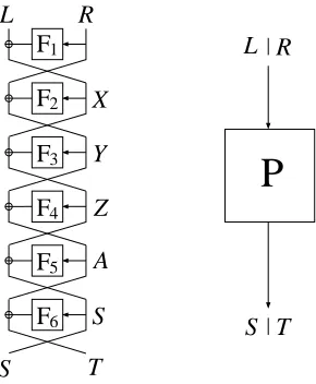
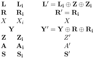
The other direction (constructing an ideal cipher from a random oracle) was left as an open problem in [9]. In this paper we solve this open problem and show that the Luby-Rackoff con-struction with 6 rounds is sufficient to instantiate an ideal cipher (see Fig. 2 for an illustration). Actually, it is easy to see that it is enough to construct a randompermutationinstead of an ideal cipher; namely, a family of 2κ independent random permutations (i.e., an ideal block cipher)
can be constructed by simply prepending a k-bit key to the inner random oracle functionsFi’s.
S T L
P
R L1
F
F
F
F
F
2
3
4
5
6
F
R
X
Y
Z
A
S
T S
Fig. 2.The Luby-Rackoff construction with 6 rounds (left), to replace a random permutationP (right).
Our result shows that the random oracle model and the ideal cipher model are actually equivalent assumptions. It seems that up to now, many cryptographers have been reluctant to use the Ideal Cipher Model and have endeavoured to work in the Random Oracle Model, arguing that the ICM is richer and carries much more structure than the ROM. Our result shows that it is in fact not the case and that designers may use the ICM when they need it without making a stronger assumption than when working in the random oracle model. However, our security reduction is quite loose, which implies that in practice large security parameters should be used in order to replace an ideal cipher by a 6-round Luby-Rackoff.
We stress that the “indifferentiable construction” notion is very different from the classical indistinguishability notion. The well known Luby-Rackoff result that 4 rounds are enough to obtain a strong pseudo-random permutation from pseudo-random functions [16], is proven under the classical indistinguishability notion. Under this notion, the adversary has only access to the input/output of the Luby-Rackoff (LR) construction, and tries to distinguish it from a random permutation; in particular it does not have access to the input/output of the inner pseudo-random functions. On the contrary, in our setting, the distinguisher can make oracle calls to the inner round functionsFi’s (see Fig. 2); the indifferentiability notion enables to accommodate
these additional oracle calls in a coherent definition.
1.1 Related Work
One of the first paper to consider having access to the inner round functions of a Luby-Rackoff is [19]; the authors showed that Luby-Rackoff with 4 rounds remains secure if adversary has oracle access to the middle two round functions, but becomes insecure if adversary is allowed access to any other round functions.
In [14] a random permutation oracle was instantiated for a specific scheme using a 4-rounds Luby-Rackoff. More precisely, the authors showed that the random permutation oracle P in the Even-Mansour [13] block-cipherEk1,k2(m) =k2⊕P(m⊕k1) can be replaced by a 4-rounds
Luby-Rackoff, and the block-cipher E remains secure in the random oracle model; for this specific scheme, the authors obtained a (much) better security bound than our general bound in this paper.
a Luby-Rackoff construction with a super-logarithmic number of rounds can replace an ideal cipher. The authors also showed that indifferentiability in the honest-but-curious model implies indifferentiability in the general model, for LR constructions with up to a logarithmic number of rounds. But because of this gap between logarithmic and super-logarithmic, the authors could not conclude about general indifferentiability of Luby-Rackoff constructions. Subsequent work by Dodis and Puniya [12] studied other properties (such as unpredictability and verifiablity) of the Luby-Rackoff construction when the intermediate values are known to the attacker.
In this paper we have an observation about indifferentiability in the honest-but-curious model: we show that general indifferentiability does not necessarily imply indifferentiability in the honest-but-curious model. More precisely, we show in Appendix B that LR constructions with up to logarithmic number of rounds are not indifferentiable from a random permutation in the honest-but-curious model, whereas our main result in this paper is that 6-rounds LR is indifferentiable from a random permutation in the general model.
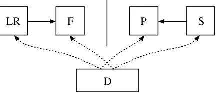
2 Definitions
In this section, we recall the notion of indifferentiability of random systems, introduced by Maurer et al.in [17]. This is an extension of the classical notion of indistinguishability, where one or more oracles are publicly available, such as random oracles or ideal ciphers.
We first motivate why such an extension is actually required. The classical notion of indis-tinguishability enables to argue that if some system S1 is indistinguishable from some other
system S2 (for any polynomially bounded attacker), then any application that usesS1 can use S2 instead, without any loss of security; namely, any non-negligible loss of security would
pre-cisely be a way of distinguishing between the two systems. Since we are interested in replacing a random permutation (or an ideal cipher) by a Luby-Rackoff construction, we would like to say that the Luby-Rackoff construction is “indistinguishable” from a random permutation. How-ever, when the distinguisher can make oracle calls to the inner round functions, one cannot say that the two systems are “indistinguishable” because they don’t even have the same interface (see Fig. 2); namely for the LR construction the distinguisher can make oracle calls to the inner functions Fi’s, whereas for the random permutation he can only query the input and receive
the output and vice versa. This contrasts with the setting of the classical Luby-Rackoff result, where the adversary has only access to the input/output of the LR construction, and tries to distinguish it from a random permutation. Therefore, an extension of the classical notion of indistinguishability is required, in order to show that some ideal primitive (like a random permutation) can be constructed from another ideal primitive (like a random oracle).
Following [17], we define an ideal primitive as an algorithmic entity which receives inputs from one of the parties and delivers its output immediately to the querying party. The ideal primitives that we consider in this paper are random oracles and random permutations (or ideal ciphers). A random oracle [1] is an ideal primitive which provides a random output for each new query. Identical input queries are given the same answer. A random permutation is an ideal primitive that contains a random permutation P :{0,1}n → {0,1}n. The ideal primitive
provides oracle access toP andP−1. Anideal cipheris an ideal primitive that models a random
block cipherE :{0,1}κ× {0,1}n→ {0,1}n. Each keyk∈ {0,1}κ defines a random permutation Ek = E(k,·) on {0,1}n. The ideal primitive provides oracle access to E and E−1; that is, on
query (0, k, m), the primitive answers c=Ek(m), and on query (1, k, c), the primitive answers m such that c=Ek(m). These oracles are available for any nand any κ.
Definition 1 ([17]). A Turing machine C with oracle access to an ideal primitive F is said to be (tD, tS, q, ε)-indifferentiable from an ideal primitive P if there exists a simulator S with oracle access to P and running in time at most tS, such that for any distinguisher D running in time at most tD and making at most q queries, it holds that:
Pr
h
DCF,F
= 1i−PrhDP,SP = 1i
< ε
CF is simply said to be indifferentiable from F if
ε is a negligible function of the security parameter n, for polynomially bounded q, tD and tS.
F P S
D LR
Fig. 3.The indifferentiability notion.
The previous definition is illustrated in Figure 3, whereP is a random permutation,C is a Luby-Rackoff construction LR, and F is a random oracle. In this paper, for a 6-round Luby-Rackoff, we denote these random oracles F1, . . . , F6 (see Fig. 2). Equivalently, one can consider
a single random oracle F and encode in the first 3 input bits which round function F1, . . . , F6
is actually called. The distinguisher has either access to the system formed by the construction
LR and the random oracle F, or to the system formed by the random permutation P and a simulator S. In the first system (left), the construction LR computes its output by making calls toF (this corresponds to the round functions Fi’s of the Luby-Rackoff); the distinguisher
can also make calls to F directly. In the second system (right), the distinguisher can either query the random permutation P, or the simulator that can make queries to P. We see that the role of the simulator is to simulate the random oracles Fi’s so that no distinguisher can tell
whether it is interacting with LR and F, or with P and S. In other words, 1) the output of
S should be indistinguishable from that of random oracles Fi’s and 2) the output of S should
look “consistent” with what the distinguisher can obtain fromP. We stress that the simulator does not see the distinguisher’s queries to P; however, it can call P directly when needed for the simulation. Note that the two systems have the same interface, so now it makes sense to require that the two systems be indistinguishable.
To summarise, in the first system the random oracles Fi are chosen at random, and a
permutation C =LR is constructed from them with a 6 rounds Luby-Rackoff. In the second system the random permutationP is chosen at random and the inner round functionsFi’s are
simulated by a simulator with oracle access toP. Those two systems should be indistinguishable, that is the distinguisher should not be able to tell whether the inner round functions were chosen at random and then the Luby-Rackoff permutation constructed from it, or the random permutation was chosen at random and the inner round functions then “tailored” to match the permutation.
It is shown in [17] that the indifferentiability notion is the “right” notion for substituting one ideal primitive with a construction based on another ideal primitive. That is, if CF
is indifferentiable from an ideal primitiveP, then CF
indifferentiable from a random permutation; this implies that such a construction can replace a random permutation (or an ideal cipher) in any cryptosystem, and the resulting scheme remains secure in the random oracle model if the original scheme was secure in the random permutation (or ideal cipher) model.
3 Attack of Luby-Rackoff with 5 Rounds
In this section we show that 5 rounds are not enough to obtain the indifferentiability property. We do this by exhibiting for the 5 rounds Luby-Rackoff (see Fig. 4) a property that cannot be obtained with a random permutation.
F1
F2
F3
F4
F5
L R
Z Y X
S
S T
Fig. 4. 5-rounds
Luby-Rackoff. Let Y and Y′
be arbitrary values, corresponding to inputs of F3 (see
Fig. 4); let Z be another arbitrary value, corresponding to input of F4. Let Z′
=F3(Y)⊕F3(Y′)⊕Z, and let:
X=F3(Y)⊕Z =F3(Y′)⊕Z′ (1) X′ =F3(Y′)⊕Z =F3(Y)⊕Z′ (2)
From X,X′
,Y and Y′
we now define four couples (Xi, Yi) as follows:
(X0, Y0) = (X, Y), (X1, Y1) = (X′, Y)
(X2, Y2) = (X′, Y′), (X3, Y3) = (X, Y′)
and we let LikRi be the four corresponding plaintexts; we have: R0 =Y0⊕F2(X0) =Y ⊕F2(X)
R1 =Y1⊕F2(X1) =Y ⊕F2(X′) R2 =Y2⊕F2(X2) =Y′⊕F2(X′) R3 =Y3⊕F2(X3) =Y′⊕F2(X)
Let Z0, Z1, Z2, Z3 be the corresponding values as input of F4; we have from (1) and (2):
Z0 =X0⊕F3(Y0) = X⊕F3(Y) =Z, Z1 =X1⊕F3(Y1) =X′⊕F3(Y) =Z′ Z2 =X2⊕F3(Y2) =X′⊕F3(Y′) =Z, Z3 =X3⊕F3(Y3) =X⊕F3(Y′) =Z′
Finally, let SikTi be the four corresponding ciphertexts; we have:
S0=Y0⊕F4(Z0) = Y ⊕F4(Z), S1=Y1⊕F4(Z1) = Y ⊕F4(Z′) S2=Y2⊕F4(Z2) =Y′⊕F4(Z), S3=Y3⊕F4(Z3) =Y′⊕F4(Z′)
We obtain the relations:
R0⊕R1⊕R2⊕R3 = 0, S0⊕S1⊕S2⊕S3= 0
Thus, we have obtained four pairs (plaintext, ciphertext) such that the xor of the right part of the four plaintexts equals 0 and the xor of the left part of the four ciphertexts also equals 0. For a random permutation, it is easy to see that such a property can only be obtained with negligible probability, when the number of queries is polynomially bounded. Thus we have shown:
Theorem 1. The Luby-Rackoff construction with 5 rounds is not indifferentiable from a
ran-dom permutation.
4 Indifferentiability of Luby-Rackoff with 6 Rounds
We now prove our main result: the Luby-Rackoff construction with 6 rounds is indifferentiable from a random permutation.
Theorem 2. The LR construction with6rounds is(tD, tS, q, ε)-indifferentiable from a random
permutation, with tS = O(q8) and ε = 224 ·q16/2n, where n is the output size of the round functions.
Note that here the distinguisher has unbounded running time; it is only bounded to ask q
queries. As illustrated in Figure 3, we must construct a simulator S such that the two systems formed by (LR, F) and (P,S) are indistinguishable. The simulator is constructed in Section 4.1, while the indistinguishability property is proved in Section 4.2.
4.1 The Simulator
We construct a simulator S that simulates the random oracles F1, . . . , F6. For each function Fi the simulator maintains an history of already answered queries. We write x ∈ Fi when x
belongs to the history of Fi, and we denote byFi(x) the corresponding output. When we need
to obtain Fi(x) and x does not belong to the history of Fi, we write Fi(x) ← y to determine
that the answer to Fi query xwill bey; we then add (x, Fi(x)) to the history of Fi. We denote
bynthe output size of the functionsFi’s. We denote byLRandLR−1 the 6-round Luby-Rackoff
construction as obtained from the functions Fi’s.
We first provide an intuition of the simulator’s algorithm. The simulator must make sure that his answers to the distinguisher’s Fi queries are coherent with the answers to P queries
that can be obtained independently by the distinguisher. In other words, when the distinguisher makes Fi queries to the simulator (possibly in some arbitrary order), the output generated by
the corresponding Luby-Rackoff must be the same as the output fromP obtained independently by the distinguisher. We stress that those P queries made by the distinguisher cannot be seen by the simulator; the simulator is only allowed to make his ownP queries (as illustrated in Fig. 3). In addition, the simulator’s answer toFi queries must be statistically close to the output of
random functions.
F1
F2
F3
F4
A
F5
S
F6
L R
Z Y X
T S
The simulator’s strategy is the following: when a “chain of 3 queries” has been made by the distinguisher, the simulator is going to define the values of all the other Fi’s corresponding to this chain, by making aP or a P−1
query, so that the output ofLR and the output of P are the same for the corresponding message. Roughly speaking, we say that we have a chain of 3 queries (x, y, z) when x, y, z are in the history of Fk, Fk+1 and Fk+2
respectively and x=Fk+1(y)⊕z.
For example, if a queryXtoF2is received, and we haveX=F3(Y)⊕Z
where Y,Z belong to the history ofF3 and F4 respectively, then the triple
(X, Y, Z) forms a 3-chain of queries. In this case, the simulator defines
F2(X) $
← {0,1}n and computes the correspondingR=Y ⊕F
2(X). It also
lets F1(R) $
← {0,1}n and computes L = X⊕F
1(R). Then it makes a P
-query to get SkT =P(LkR). It also computes A=Y ⊕F4(Z). The values
of F5(A) and F6(S) are then “adapted” so that the 6-round LR and the
random permutation provide the same output, i.e. the simulator defines
F5(A)←Z⊕S andF6(S)←A⊕T, so thatLR(LkR) =P(LkR) =SkT. In
summary, given a F2 query, the simulator looked at the history of (F3, F4)
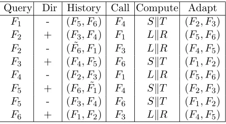
More generally, given a query to Fk, the simulator proceeds according to Table 1 below;
we denote by + for looking downward in the LR construction and by − for looking upward. The simulator must first simulate an additional call toFi (column “Call”). Then the simulator
can compute either LkR or SkT (as determined in column “Compute”). Given LkR (resp.
SkT) the simulator makes a P-query (resp. a P−1-query) to obtain SkT = P(LkR) (resp. LkR=P−1
(SkT)). Finally Table 1 indicates the index j for which the output of (Fj, Fj+1) is
adapted (column “Adapt”).
Query Dir History Call Compute Adapt
F1 - (F5, F6) F4 SkT (F2, F3) F2 + (F3, F4) F1 LkR (F5, F6) F2 - ( ˜F6, F1) F3 LkR (F4, F5) F3 + (F4, F5) F6 SkT (F1, F2) F4 - (F2, F3) F1 LkR (F5, F6) F5 + (F6,F˜1) F4 SkT (F2, F3) F5 - (F3, F4) F6 SkT (F1, F2) F6 + (F1, F2) F3 LkR (F4, F5)
Table 1. Simulator’s behaviour.
For Line (F2,+) in Table 1, given a queryX toF2, the simulator must actually consider all
3-chains formed by (X, Y, Z), whereY ∈F3 and Z ∈F4; formally, one defines the following set:
Chain(+1, X,2) ={(Y, Z)∈(F3, F4) |X=F3(Y)⊕Z}
where +1 corresponds to looking downward in the Luby-Rackoff construction. Similarly for Line (F3,+):
Chain(+1, Y,3) ={(Z, A)∈(F4, F5) |Y =F4(Z)⊕A}
Symmetrically for Lines (F5,−) and (F4,−):
Chain(−1, A,5) ={(Y, Z)∈(F3, F4) |A=F4(Z)⊕Y}
Chain(−1, Z,4) ={(X, Y)∈(F2, F3)|Z =F3(Y)⊕X}
Additionally with Line (F6,+) one must consider the 3-chains obtained from aF6 queryS
and looking in (F1, F2) history:
Chain(+1, S,6) =n(R, X)∈(F1, F2) | ∃T, P(F1(R)⊕XkR) =SkT
o
(3)
and symmetrically with Line (F1,−) the 3-chains obtained from a F1 query R and looking in
(F5, F6) history:
Chain(−1, R,1) =n(A, S)∈(F5, F6)| ∃L, P−1(SkF6(S)⊕A) =LkR
o
(4)
With Lines (F2,−) and (F5,+), one must also consider the 3-chains associated with (F1, F6)
history, obtained either from a F2 query X or a F5 query A. Given aF2 query X, we consider
all R ∈ F1, and for each corresponding L = X⊕F1(R), we compute SkT = P(LkR) and
determine whether S ∈ F6. Additionally, we also consider “virtual” 3-chains, where S /∈ F6,
but S is such that P(L′
kR′
) =SkT′
for some (R′
, X′
) ∈(F1, F2), with L′ =X′⊕F1(R′) and X′
6
=X. Formally, we denote :
Chain(−1, X,2) =n(R, S)∈(F1,F˜6)| ∃T, P(X⊕F1(R)kR) =SkT
o
where ˜F6 inChain(−1, X,2) is defined as:
˜
F6=F6∪
n
S | ∃T′,(R′, X′)∈(F1, F2\ {X}), P(X′⊕F1(R′)kR′) =SkT′
o
and symmetrically for Line (F5,+):
Chain(+1, A,5) =n(R, S)∈( ˜F1, F6)| ∃L, P−1(SkA⊕F6(S)) =LkR
o
(6)
˜
F1 =F1∪
n
R | ∃L′
,(A′
, S′
)∈(F5\ {A}, F6), P−1(S′kA′⊕F6(S′)) =L′kR
o
When the simulator receives a query x for Fk from the distinguisher, it then proceeds as
follows:
Query(x, k):
1. If x is in the history ofFk then go to step 4.
2. Let Fk(x) $
← {0,1}n
3. Call ChainQuery(x, k) 4. Return Fk(x).
The ChainQuery algorithm is used to handle all possible 3-chains created by the operation
Fk(x) $
← {0,1}n at step 2:
ChainQuery(x, k):
1. If k∈ {1,2,5,6}, then call XorQuery1(x, k)
2. If k∈ {1,3,4,6}, then call XorQuery2(x, k)
3. If k∈ {3,4}, then call XorQuery3(x, k)
4. Let U ← ∅
5. If k∈ {2,3,5,6}:
(a) For all (y, z)∈Chain(+1, x, k), let U ←U ∪CompleteChain(+1, x, y, z, k). 6. If k∈ {1,2,4,5}:
(a) For all (y, z)∈Chain(−1, x, k), let U ←U ∪CompleteChain(−1, x, y, z, k). 7. For all (x′
, k′
)∈U, call ChainQuery(x′
, k′ ).
TheCompleteChain(b, x, y, z, k) works as follows: it computes the messageLkR orSkT that corresponds to the 3-chain (x, y, z) given as input, without querying (Fj, Fj+1), wherej is the
index given in Table 1 (column “Adapt”). IfLkR is first computed, then the simulator makes a
P query to obtainSkT =P(LkR); similarly, ifSkT is first computed, then the simulator makes aP−1
query to obtainLkR=P−1
(SkT). The output of functions (Fj, Fj+1) is adapted so that
LR(LkR) = SkT. The CompleteChain algorithm eventually returns the set of variables which were added in the history of the Fi’s; then for each of these variables theChainQueryalgorithm
is recursively applied.
CompleteChain(b, x, y, z, k): 1. Let U ← ∅
2. If (b, k) = (−1,2) andz /∈F6, then let F6(z)← {0,1}n and U ←U ∪ {(z,6)}
3. If (b, k) = (+1,5) andy /∈F1, then let F1(y)← {0,1}n and U ←U∪ {(y,1)}
4. Given (b, k) and from Table 1:
(a) Determine the index iof the additional call to Fi (column “Call”), and let xi be the
corresponding input to Fi.
(b) Determine whether LkR orSkT must be computed first.
(c) Determine the indexj for adaptation at (Fj, Fj+1) (column “Adapt”).
6. Compute the message LkR orSkT corresponding to the 3-chain (x, y, z).
7. IfLkRhas been computed, make aP query to get SkT =P(LkR); otherwise, make aP−1
query to get LkR=P−1(SkT).
8. Now all input values (x1, . . . , x6) to (F1, . . . , F6) corresponding to the 3-chain (x, y, z) are
known. Additionally let x0 ←Land x7←T.
9. If xj is in the history of Fj orxj+1 is in the history ofFj+1, abort.
10. Define Fj(xj)←xj−1⊕xj+1
11. Define Fj+1(xj+1)←xj⊕xj+2
12. Let U ←U ∪ {(xj, j),(xj+1, j+ 1)}
13. Return U.
Finally, theXorQuery1(x, k),XorQuery2(x, k) andXorQuery3(x, k) algorithms are defined as
follows:
XorQuery1(x, k):
1. If k= 5, then let A′={x⊕R
1⊕R2 ∈/F5 |R1, R2 ∈F1 and R1 6=R2}
2. If k= 1, then let A′
={A⊕x⊕R2 ∈/ F5 |A∈F5 and R2∈F1}
3. If k= 5 or k= 1, then for allA′∈ A′ :
(a) If for some S∈F6,P−1(SkF6(S)⊕A′) =LkR withR∈F1:
i. LetF5(A′)← {0,1}n
ii. Call ChainQuery(A′
,5) 4. If k= 2, then let X′
={x⊕S1⊕S2∈/ F2 |S1, S2 ∈F6 and S1 6=S2}
5. If k= 6, then let X′
={X⊕x⊕S2 ∈/ F2 |X ∈F2 and S2 ∈F6}
6. If k= 2 or k= 6, then for allX′ ∈ X′ :
(a) If for some R∈F1,P(F1(R)⊕X′kR) =SkT withS ∈F6:
i. LetF2(X′)← {0,1}n
ii. Call ChainQuery(X′
,2)
XorQuery2(x, k):
1. Let M={(L, R, Z, A, S) |LkR=P−1
(SkA⊕F6(S)), Z =F5(A)⊕S, A∈F5, S ∈F6, R /∈ F1}
2. For all (L, R, Z, A, S)∈ M: (a) If k= 6 and for someZ′
∈F4\ {Z},P(L⊕Z⊕Z′kR) =xkT for some T, or if k= 3
and P(L⊕x⊕ZkR) =S′kT for someT withS′ ∈F
6:
i. LetF1(R)← {0,1}n
ii. Call ChainQuery(R,1)
3. LetC ={S, T, R, X, Y)|SkT =P(X⊕F1(R)kR), Y =F2(X)⊕R, R∈F1, X∈F2, S /∈F6}
4. For all (S, T, R, X, Y)∈ C: (a) Ifk= 1 and for someY′
∈F3\ {Y},P−1(SkT⊕Y ⊕Y′) =Lkxfor someL, or ifk= 4
and P−1
(SkT ⊕x⊕Y) =LkR′
for someL withR′ ∈
F1:
i. LetF6(S)← {0,1}n
ii. Call ChainQuery(S,6)
XorQuery3(x, k):
1. LetR={(Y, R1, R2)|Z1 =F5(A1)⊕S1, Z1 ∈F4, A1 ∈F5, S1∈F6, Y =F4(Z1)⊕A1, Y /∈ F3, A2 =F4(Z2)⊕Y, Z2 ∈ F4, A2 ∈F5, S2 =F5(A2)⊕Z2, S2 ∈F6, P−1(S1kF6(S1)⊕ A1) =L1kR1, P−1(S2kF6(S2)⊕A2) =L2kR2}
2. If k= 3 and for some (Y, R1, R2)∈ R,x=Y ⊕R1⊕R2:
(a) LetF3(Y)← {0,1}n
3. LetS ={(Z, S1, S2)|Y1 =F2(X1)⊕R1, Y1 ∈F3, X1∈F2, R1 ∈F1, Z =F3(Y1)⊕X1, Z /∈ F4, X2=F3(Y2)⊕Z, Y2 ∈F3, X2∈F2, R2 =F2(X2)⊕Y2, R2 ∈F1, P(F1(R1)⊕X1kR1) = S1kT1, P(F1(R2)⊕X2kR2) =S2kT2}
4. If k= 4 and for some (Z, S1, S2)∈ S,x=Z⊕S1⊕S2:
(a) LetF4(Z)← {0,1}n
(b) Call ChainQuery(Z,4)
Additionally the simulator maintains an upper bound Bmax on the size of the history of
each of the Fi’s; if this bound is reached, then the simulator aborts; the value of Bmax will be
determined later. This terminates the description of the simulator.
We note that all lines in Table 1 are necessary to ensure that the simulation of the Fi’s
is coherent with what the distinguisher can obtain independently from P. For example, if we suppress the line (F2,+) in the table, the distinguisher can make a query forZ to F4, then Y
to F3 andX =F3(Y)⊕Z toF2, thenA=F4(Z)⊕Y to F5 and since it is not possible anymore
to adapt the output of (F1, F2), the simulator fails to provide a coherent simulation.
We also note that a simulator would necessarily fail for a 5-rounds LR: using the same approach as in Section 3, the distinguisher can ask F3(Y) andF3(Y′), then letX,X′ such that Z = X⊕F3(Y) = X′ ⊕F3(Y′) which gives Z′ = X′ ⊕F3(Y) = X ⊕F3(Y′); when queried
for F4(Z), the simulator can adapt the answer ofF4(Z) corresponding to chain (X, Y, Z), and
adapt the answer ofF2(X′) for chain (X′, Y′, Z); however, when queried forF4(Z′), the simulator
cannot adapt the answer ofF4(Z′) for both chains (X, Y′, Z′) and (X′, Y, Z′). We also note that
one could have taken 12 lines in Table 1 instead of 8, by taking both directions + and − for each of the Fi’s, and without considering “virtual” 3-chains in equations (5) and (6); however
in this case it seems harder to bound the simulator’s running time.
Our simulator makes recursive calls to theQueryand ChainQueryalgorithms. The simulator aborts when the history size of one of the Fi’s is greater thanBmax. Therefore we must prove
that despite these recursive calls, this bound Bmax is never reached, except with negligible
probability, for Bmax polynomial in the security parameter. The main argument is that the
number of 3-chains in the sets Chain(b, x, k) that involve theP permutation (equations (3), (4), (5) and (6)), must be upper bounded by the number ofP/P−1
-queries made by the distinguisher, which is upper bounded byq. This gives an upper bound on the number of recursive queries to
F3,F4, which in turn implies an upper bound on the history of the otherFi’s. Additionally, one
must show that the simulator never aborts at Step 9 in the CompleteChain algorithm, except with negligible probability. This is summarised in the following lemma:
Lemma 1. Let qbe the maximum number of queries made by the distinguisher and let Bmax =
5q2. The simulatorS runs in timeO(q8), and aborts with probability at most215·q10/2n, while making at most 210·q8 queries toP or P−1.
Proof. See Appendix A
4.2 Indifferentiability
We now proceed to prove the indifferentiability result. As illustrated in Figure 3, we must show that given the previous simulator S, the two systems formed by (LR, F) and (P,S) are indistinguishable.
We consider a distinguisher D making at most q queries to the system (LR, F) or (P,S) and outputting a bitγ. We define a sequenceGame0,Game
1,. . .of modified distinguisher games.
In the first game Game0, the distinguisher interacts with the system formed by the random
P S
D D
LR F
Game 3 Game 0
P
D F
Game 1 P S’
T
D LR
F
Game 2 S’
T’
Fig. 5.Sequence of games for proving indifferentiability.
modified so that in the last game the distinguisher interacts with (LR, F). We denote bySi the
event in game ithat the distinguisher outputs γ = 1.
Game0: the distinguisher interacts with the simulatorS and the random permutation P. Game1: we make a minor change in the wayFiqueries are answered by the simulator, to prepare
a more important step in the next game. InGame0 we have that aFi query forxcan be answered
in two different ways: either Fi(x) $
← {0,1}, or the value Fi(x) is “adapted” by the simulator.
In Game1, instead of letting Fi(x) ← {$ 0,1}, the new simulator S′ makes a query to a random
oracle Fi which returnsFi(x); see Fig. 5 for an illustration. Since we have simply replaced one
set of random variables by a different, but identically distributed, set of random variables, we have:
Pr[S0] = Pr[S1]
Game2: we modify the way P and P−1 queries are answered. Instead of returningP(LkR) with
random permutation P, the system returns LR(LkR) by calling the random oracles Fi’s (and
similarly forP−1 queries).
We must show that the distinguisher’s view has statistically close distribution inGame1 and Game2. For this, we consider the subsystem T with the random permutation P/P−1 and the
random oracles Fi’s in Game1, and the subsystem T′ with Luby-Rackoff LR and random oracle Fi’s in Game2 (see Fig. 5). We show that the output of systemsT and T′ is statistically close;
this in turn shows that the distinguisher’s view has statistically close distribution in Game1 and Game2.4
In the following, we assume that the distinguisher eventually makes a sequence ofFi-queries
corresponding to all previous P/P−1 queries made by the distinguisher; this is without loss of
generality, because from any distinguisher D we can build a distinguisher D′
with the same output that satisfies this property.
The outputs toFi queries provided by subsystemT inGame1 and by subsystemT′ inGame2
are the same, since in both cases these queries are answered by random oracles Fi. Therefore,
we must show that the output to P/P−1
queries provided by T and T′
have statistically close distribution, when the outputs to Fi queries provided byT orT′ are fixed.
We can distinguish two types of P/P−1
queries toT orT′ :
– Type I: P/P−1
queries made by the distinguisher, or by the simulator during execution of the CompleteChain algorithm. From Lemma 1 there are at most Bmax +q ≤ 6q2 such
queries.
4
We do not claim that subsystems T and T′
– Type II: P/P−1
queries made by the simulator when computing the sets Chain(+1, S,6),
Chain(−1, R,1), Chain(+1, A,5) and Chain(−1, X,2) and executing algorithms XorQuery1,
XorQuery2 and XorQuery3, which are not of Type I. From Lemma 1 there are at most
QP = 210·q8 such queries.
We first consider Type I queries. Recall that the distinguisher is assumed to eventually make all the Fi queries corresponding to his P/P−1 queries; consequently at the end of the
distin-guisher’s queries, theCompleteChainalgorithm has been executed for all 3-chains corresponding to P/P−1 queries of Type I. We consider one suchP query LkR (the argument for P−1 query
is similar) of Type I. InGame2 the answer SkT can be written as follows:
(S, T) = (L⊕r1⊕r3⊕r5, R⊕r2⊕r4⊕r6) (7)
where r1 = F1(R), r2 = F2(X), r3 = F3(Y), r4 = F4(Z), r5 = F5(A) and r6 = F6(S), and
(X, Y, Z, A) are defined in the usual way.
Letjbe the index used at steps 10 and 11 of the correspondingCompleteChainexecution, and letxj,xj+1 be the corresponding inputs. If the simulator does not abort duringCompleteChain,
this implies that the values rj =Fj(xj) andrj+1=Fj+1(xj+1) have not appeared before in the
simulator’s execution. This implies that rj =Fj(xj) and rj+1 =Fj+1(xj+1) have not appeared
in a previous P/P−1-query (since otherwise it would have been defined in the corresponding
CompleteChain execution), and moreover Fj(xj) and Fj+1(xj+1) have not been queried before
to subsystem T′
. Moreover since the values rj =Fj(xj) andrj+1 =Fj+1(xj+1) are defined by
the simulator at steps 10 and 11 ofCompleteChain, these values will not be queried later toT′. Therefore we have that rj =Fj(xj) andrj+1 =Fj+1(xj+1) are not included in the subsystem T′
output; T′
output can only include randoms in (r1, . . . , rj−1, rj+2, . . . , r6). Therefore, we
obtain from equation (7) that for fixed randoms (r1, . . . , rj−1, rj+2, . . . , r6) the distribution of SkT =LR(LkR) in Game2 is uniform in {0,1}2n and independent from the output of previous
P/P−1
queries.
InGame1, the output to queryLkRisSkT =P(LkR); since there are at mostq+Bmax ≤6·q2
Type I queries to P/P−1
, the statistical distance between P(LkR) and LR(LkR) is at most 6·q2/22n. This holds for a singleP/P−1
query of Type I. Since there are at most 6·q2 such queries, we obtain the following statistical distance δ between outputs of systemsT and T′
to Type I queries, conditioned on the event that the simulator does not abort:
δ≤6·q2·6·q 2
22n ≤
36·q4
22n (8)
We now considerP/P−1 queries of Type II; from Lemma 1 there are at mostQ
P = 210·q8
such queries. We first consider the sets Chain(+1, S,6) andChain(−1, X,2):
Chain(+1, S,6) =n(R, X)∈(F1, F2) | ∃T, P(F1(R)⊕XkR) =SkT
o
Chain(−1, X,2) =n(R, S)∈(F1,{0,1}n) | ∃T, P(X⊕F1(R)kR) =SkT and
(S ∈F6, or∃T′, (R′, X′)6= (R, X)∈(F1, F2), P(X′⊕F1(R′)kR′) =SkT′)
o
and we consider a corresponding query LkR to P, where L = F1(R)⊕X. By definition this
query is not of Type I, so noCompleteChainexecution has occurred corresponding to this query. Given (R, X)∈Chain(+1, S,6) or for (R, S) ∈Chain(−1, X,2), we let Y =F2(X)⊕R. If Y is
not in the history of F3, we let F3(Y) $
← {0,1}n; in this case, Z =X⊕F
3(Y) has the uniform
distribution in {0,1}n; this implies that Z belongs to the history of F
most |F4|/2n ≤ 2q/2n. If Y belongs to the history of F3, then we have that Z cannot be in
the history of F4, otherwise 3-chain (X, Y, Z) would already have appeared in CompleteChain
algorithm, from Line (F2,+) and (F4,−) in Table 1. Therefore, we have that for allP queries LkRof Type II, no corresponding value ofZ belongs to the history ofF4, except with probability
at mostQP ·2q/2n.
We now consider the sequence (Li, Ri) of distinct P-queries of Type II corresponding to
the previous sets Chain(+1, S,6) andChain(−1, X,2). We must show that inGame2 the output
(Si, Ti) provided byT′ has a distribution that is statistically close to uniform, when the outputs
to Fi queries provided by T′ are fixed. We consider the corresponding sequence of (Yi, Zi); as
explained previously, noZi belongs to the simulator’s history ofF4, except with probability at
most QP ·2q/2n. We claim that F4(Zi)⊕Yi 6= F4(Zj)⊕Yj for all 1 ≤ i < j ≤ QP, except
with probability at most (QP)2/2n. We distinguish two cases. If Zi =Zj for some i < j, then F4(Zi)⊕Yi=F4(Zj)⊕Yj impliesYi=Yj, which gives (Li, Ri) = (Lj, Rj), a contradiction since
we have assumed the (Li, Ri) queries to be distinct. If Zi 6=Zj for all i < j, then we have that F4(Zi)⊕Yi =F4(Zj)⊕Yj happens with probability at most 2−n; since there are at most (QP)2
such i, j, we have that F4(Zi)⊕Yi =F4(Zj)⊕Zj for some i < j happens with probability at
most (QP)2/2n.
This implies that the elements Ai = Yi ⊕F4(Zi) are all distinct, except with probability
at most (QP)2/2n. Therefore elements Si = Zi ⊕ F5(Ai) are uniformly and independently
distributed in {0,1}n; this implies that elements S
i are all distinct, except with probability at
most (QP)2/2n, which implies that elements Ti =Ai⊕F6(Si) are uniformly and independently
distributed in {0,1}n. For each (S
i, Ti), the statistical distance with P(LikRi) in Game1 is
therefore at most QP/22n. The previous arguments are conditioned on the event that no Ai
or Si belongs to the simulator’s history for F5 and F6, which for each Ai or Si happens with
probability at most Bmax/2n. The reasoning for the sets Chain(−1, R,1), Chain(+1, A,5) is
symmetric so we omit it. The reasoning for the XorQuery1, XorQuery2 and XorQuery3 calls is
also the same so we omit it. We obtain that the statistical distance δ2 between the output
of Type II P/P−1
queries in Game1 and Game2 is at most (conditioned on the event that the
simulator does not abort):
δ2≤2·
QP ·2q
2n + 2·
(QP)2
2n +
(QP)2
22n +
QP ·Bmax
2n
!
≤ 2 22·q16
2n (9)
Let denote by Abort the event that the simulator aborts in Game1; we obtain from Lemma 1
and inequalities (8) and (9) :
|Pr[S2]−Pr[S1]| ≤Pr[Abort] +δ+δ2 ≤
215·q10
2n +
36·q4
22n +
222·q16
2n ≤
223·q16
2n
Game3: the distinguisher interacts with random system (LR, F). We have that system (LR, F)
provides the same outputs as the system inGame2 except if the simulator fails inGame2. Namely,
when the output values of (Fj, Fj+1) are adapted (steps 10 and 11 ofCompleteChainalgorithm),
the valuesFj(xj) andFj+1(xj+1) are the same as the one obtained directly from random oracles Fj and Fj+1, because inGame2 the P/P−1 queries are answered usingLR/LR−1. Let denote by
Abort2 the event that simulator aborts in Game2; we have:
Pr[Abort2]≤Pr[Abort] +δ+δ2 ≤
223·q16
2n
which gives:
|Pr[S3]−Pr[S2]| ≤Pr[Abort2]≤ 2 23·
q16
From the previous inequalities, we obtain the following upper bound on the distinguisher’s advantage:
|Pr[S3]−Pr[S0]| ≤ 2 24·
q16
2n
which terminates the proof of Theorem 2.
5 Conclusion and Further Research
We have shown that the 6 rounds Feistel construction is indifferentiable from a random permu-tation, a problem that was left open in [9]. This shows that the random oracle model and the ideal cipher model are equivalent models. A natural question is whether our security bound in
q8/2n is optimal or not. We are currently investigating:
– a better bound for 6 rounds (or more),
– best exponential attacks against 6 rounds (or more),
– other models of indifferentiability with possibly simpler proofs.
Acknowledgements: we would like to thank the anonymous referees of Crypto 2008 for their
useful comments.
References
1. M. Bellare and P. Rogaway,Random oracles are practical: A paradigm for designing efficient protocols, In Proceedings of the 1st ACM Conference on Computer and Communications Security (1993), 62 -73. 2. M. Bellare and P. Rogaway, The exact security of digital signatures - How to sign with RSA and Rabin.
Proceedings of Eurocrypt’ 96, LNCS vol. 1070, Springer-Verlag, 1996, pp. 399-416.
3. M. Bellare and P. Rogaway,Optimal Asymmetric Encryption, Proceedings of Eurocrypt’ 94, LNCS vol. 950, Springer-Verlag, 1994, pp. 92-111.
4. J. Black,The Ideal-Cipher Model, Revisited: An Uninstantiable Blockcipher-Based Hash Function, Proceed-ings of FSE 2006: 328-340.
5. J. Black, P. Rogaway, T. Shrimpton, Black-Box Analysis of the Block Cipher-Based Hash-Function Con-structions from PGV, in Advances in Cryptology - CRYPTO 2002, California, USA.
6. D. Boneh, C. Gentry, H. Shacham, and B. Lynn,Aggregate and Verifiably Encrypted Signatures from Bilinear Maps. In proceedings of Eurocrypt 2003, LNCS 2656, pp. 416-432, 2003
7. R. Canetti, O. Goldreich, and S. Halevi, The random oracle methodology, revisited, In Proceedings of the 30th ACM Symposium on the Theory of Computing (1998), ACM Press, pp. 209 -218.
8. D. Chang, S. Lee, M. Nandi and M. Yung,Indifferentiable Security Analysis of Popular Hash Functions with Prefix-Free Padding. Proceedings of ASIACRYPT 2006: 283-298.
9. J.S. Coron, Y. Dodis, C. Malinaud and P. Puniya, Merkle-Damg˚ard Revisited: How to Construct a Hash Function. Proceedings of CRYPTO 2005: 430-448.
10. A. Desai,The security of all-or-nothing encryption: Protecting against exhaustive key search, In Advances in Cryptology - Crypto’ 00 (2000), LNCS vol. 1880, Springer-Verlag.
11. Y. Dodis and P. Puniya, On the Relation Between the Ideal Cipher and the Random Oracle Models. Pro-ceedings of TCC 2006: 184-206.
12. Y. Dodis, P. Puniya,Feistel Networks Made Public, and Applications. In Proceedings of EUROCRYPT 2007, LNCS vol. 4515, Springer-Verlag, 2007, pp. 534-554.
13. S. Even and Y. Mansour,A construction of a cipher from a single pseudorandom permutation, In Advances in Cryptology - ASIACRYPT’ 91 (1992), LNCS vol. 739, Springer-Verlag, pp. 210 -224.
14. C. Gentry and Z. Ramzan, Eliminating Random Permutation Oracles in the Even-Mansour Cipher, In Advances in Cryptology - ASIACRYPT 2004, Springer-Verlag.
15. J. Kilian and P. Rogaway,How to protect DES against exhaustive key search (An analysis of DESX), Journal of Cryptology 14, 1 (2001), 17 -35.
16. M. Luby and C. Rackoff,How to construct pseudorandom permutations from pseudorandom functions, SIAM Journal of Computing, 17(2):373-386, 1988.
18. J. Patarin, Pseudorandom Permutations Based on the DES Scheme, EUROCODE ’90, LNCS vol. 514, Springer, 1990, pp. 193-204.
19. Z. Ramzan and L. Reyzin,On the Round Security of Symmetric-Key Cryptographic Primitives, Proceedings of CRYPTO 2000, Springer-Verlag.
A Proof of Lemma 1
A.1 Simulator’s Running Time
We first give an upper bound on the total number of executions of CompleteChain(b, x, y, z, k) for (b, k)∈ {(+1,6),(−1,2),(−1,1),(+1,5)}. We first consider the set:
Chain(+1, S,6) =n(R, X)∈(F1, F2) | ∃T, P(X⊕F1(R)kR) =SkT
o
that generates executions of CompleteChain(+1, S, R, X,6). We denote by cbad6 the event that
CompleteChain(+1, S, R, X,6) was called while X ⊕F1(R)kR has not appeared in a P/P−1
query made by the distinguisher. Similarly, considering the set:
Chain(−1, X,2) =n(R, S)∈(F1,F˜6) | ∃T, P(X⊕F1(R)kR) =SkT
we denote bycbad2 the event thatCompleteChain(−1, X, R, S,2) was called whileX⊕F1(R)kR
has not appeared in a P/P−1
query made by the distinguisher. Symmetrically, we denote by
cbad1 andcbad5the events forCompleteChain(−1, R, A, S,1) andCompleteChain(+1, A, R, S,5).
We denote cbad=cbad1∨cbad2∨cbad5∨cbad6.
Lemma 2. The total number of executions of CompleteChain(b, x, y, z, k) for (b, k)∈ {(+1,6),
(−1,2), (−1,1),(+1,5)} is upper bounded by the number of P/P−1 queries made by the distin-guisher, unless event cbad occurs, which happens with probability at most:
Pr[cbad]≤ 5·(Bmax) 4
2n (10)
Proof. If event cbad has not occurred, then the distinguisher has made a P/P−1 query
corre-sponding to all pairs (x, y) in CompleteChain(b, x, y, z, k) for (b, k) ∈ {(+1,6), (−1,2), (−1,1), (+1,5)}; since the distinguisher makes at mostq queries, the total number of executions is then upper bounded by q.
We first consider eventcbad6 corresponding toChain(+1, S,6). IfLkRwithL=X⊕F1(R)
has never appeared in a P/P−1
query made by the distinguisher, then the probability that
P(LkR) = SkT for some T is at most 2−n. For a single S query to F
6, the probability that
cbad6 occurs is then at most|F1| · |F2|/2n ≤(Bmax)2/2n. Since there has been at most Bmax
such queries toF6, this gives:
Pr[cbad6]≤
(Bmax)3
2n
Symmetrically, the same bound holds for event cbad1.
Similarly, for event cbad2, if the distinguisher has not made a query for P(LkR) where L = X⊕F1(R), then the probability that P(LkR) = SkT with S ∈ F˜6 is at most |F˜6|/2n,
where |F˜6| ≤ |F6|+|F1| · |F2| ≤2·(Bmax)2. For a singleX query, this implies that eventcbad2
occurs with probability at most |F1| · |F˜6|/2n; since there are at most Bmax such queries, this
gives:
Pr[cbad2]≤Bmax·
|F1| · |F˜6|
2n ≤
2·(Bmax)4
2n
Symmetrically, the same bound holds for event cbad5. From the previous inequalities we obtain
Using a similar argument, we now give an upper-bound on the number of additional Fi
calls made by the XorQuery1, XorQuery2 and XorQuery3 algorithms. For XorQuery1, we denote
by xbad1 the event that F5(A′) $
← {0,1}n occurred while SkF
6(S)⊕A′ has never appeared
in a P/P−1 query made by the distinguisher. We denote by xbad′
1 the symmetric event for F2(X′)
$
← {0,1}n. ForXorQuery
2, we denote byxbad2 the event thatF1(R) $
← {0,1}n occurred
whileL⊕Z⊕Z′
orL⊕x⊕Z′
has never appeared in aP/P−1
query made by the distinguisher. We denote by xbad′2 the symmetric event for F6(S)
$
← {0,1}n. For XorQuery
3, we denote by
xbad3 the event that F3(Y) $
← {0,1}n occurred while S
1kF6(S1)⊕A1 orS2kF6(A2)⊕A2 has
never appeared in aP/P−1
query. We denote byxbad′3the symmetric event forF4(Z) $
← {0,1}n.
We let xbad=xbad1∨xbad′1∨xbad2∨xbad′2∨xbad3∨xbad′3.
Lemma 3. The total number of Fi(x)
$
← {0,1}n executions made by algorithms XorQuery 1,
XorQuery2 and XorQuery3 is upper-bounded by the number of P/P−1 queries made by the dis-tinguisher, unless event xbad occurs, with:
Pr[xbad]≤3·(Bmax) 5
2n (11)
Proof. As previously, if eventxbad has not occurred, then the distinguisher has made aP/P−1
query corresponding to all additional Fi calls made by XorQuery1, XorQuery2 and XorQuery3;
the number of additionalFi calls is then upper-bounded by the number ofP/P−1 queries made
by the distinguisher.
ForXorQuery1(x, k), if the distinguisher has not made a P−1 query for SkF6(S)⊕A′, then
the probability that P(SkF6(S)⊕A′) =LkR with R∈F1 is at most |F1|/2n. This holds for a
given query x, a given S ∈F6 and a given A′ ∈ A′. Since there are at most Bmax such queries x, this gives:
Pr[xbad1]≤Bmax·
|F1| · |F6| · |A′|
2n ≤
(Bmax)5
2n
and the same bound holds for event xbad′1. Using the same arguments for XorQuery2, we have:
Pr[xbad2]≤ |M| ·
(Bmax)2
2n ≤
(Bmax)4
2n
and the same bound holds for xbad′2. Finally for XorQuery3, we have:
Pr[xbad3]≤ |R| ·
(2q)
2n ≤
(Bmax)4
2n
and the same bound holds for xbad′3. From these inequalities we get (11). ⊓⊔
Lemma 4. TakingBmax = 5·q2, the history size of the simulator Fi’s does not reach the bound
Bmax, unless event bad=cbad∨xbad occurs, which happens with probability at most:
Pr[bad]≤ 2 14
·q10
2n (12)
Proof. The 3-chains from Lines (F6,+), (F2,−), (F1,−) and (F5,+) in Table 1 are the only
ones which can generate recursive calls to F3 and F4, since the other 3-chains from Lines
(F2,+), (F3,+), (F4,−) and (F5,−) always include elements in F3 and F4 histories; moreover
the XorQuery1 and XorQuery2 algorithms do not generate calls to F3 and F4. From Lemma
{(+1,6),(−1,2),(−1,1),(+1,5)} is upper bounded by the number of P/P−1
queries made by the distinguisher, unless event cbad occurs. Moreover from Lemma 3 the number of recursive queries made by XorQuery3 algorithm toF3 and F4 is upper-bounded by the number of P/P−1
queries made by the distinguisher, unless event xbad occurs. Therefore, the total number of executions of CompleteChain(b, x, y, z, k) with (b, k)∈ {(+1,6),(−1,2),(−1,1),(+1,5)} and ex-ecutions of XorQuery3, is also upper bounded by the number of P/P−1 queries made by the
distinguisher (unless event bad=cbad∨xbad occurs), which is upper bounded by q. This im-plies that at most qrecursive queries toF3 andF4 can occur, unless event badoccurs. Since the
distinguisher himself makes at mostq queries toF3 and F4, the total size ofF3 andF4 histories
in the simulator is then upper bounded by q+q = 2·q.
The 3-chains from Lines (F2,+), (F3,+), (F4,−) and (F5,−) always include elements from
both F3 and F4 histories. Therefore, the number of such 3-chains is upper bounded by (2q)2 =
4·q2. This implies that the simulator makes at most 4q2 recursive queries to F1, F2, F5 and F6 when dealing with these 3-chains. Moreover from Lemma 3 the number of recursive queries
made by XorQuery1 and XorQuery2 algorithms to F1, F2, F5 and F6 is upper-bounded by the
number ofP/P−1
queries made by the distinguisher, which is upper-bounded byq, unless event
xbad occurs. Since the distinguisher can make at most q direct calls to F1,F2,F5 and F6, the
history size of F1,F2,F5 andF6 remains upper-bounded by 4q2+q+q <5q2, unless eventbad
occurs. Therefore, taking:
Bmax = 5·q2 (13)
we obtain that the simulator does not reach the bound Bmax, except if event badoccurs; from
inequalities (10), (11) and equation (13), we obtain (12). ⊓⊔
Lemma 5. With Bmax = 5·q2, the simulator makes at most 210·q8 queries to P/P−1 and
runs in time O(q8).
Proof. The simulator makes queries toP/P−1
is the following three cases:
1. Computation of sets Chain(+1, S,6),Chain(−1, R,1),Chain(+1, A,5) andChain(−1, X,2). 2. Completion of a 3-chain with CompleteChainalgorithm.
3. Algorithms XorQuery1,XorQuery2 and XorQuery3
Since the history size of theFi’s is upper bounded byBmax = 5·q2, the number ofP/P−1
-queries for Case 1 is at most Q1 = 4·(Bmax)2. Since CompleteChain algorithm gets called at
mostBmax times, the number ofP/P−1-queries for Case 2 is at mostQ2 =Bmax. Finally since
the history size of the Fi’s is upper bounded by Bmax = 5·q2, the number of P/P−1-queries
for Case 3 is at most Q3= (Bmax)4.
Therefore, the numberQP of P/P−1-queries made by the simulator is at most:
QP ≤Q1+Q2+Q3≤4·(Bmax)2+Bmax+ (Bmax)4 ≤210·q8 (14)
From this we have that the simulator runs in time O(q8). ⊓⊔
This completes the first part of the proof of Lemma 1.
A.2 Simulator’s Failure Probability
We must show that the simulator never aborts at Step 9 in theCompleteChainalgorithm, except with negligible probability. We denote by Abort9 the event that the simulator aborts at Step 9
Lemma 6. With Bmax = 5·q2, the event Abort9 occurs with probability at most :
Pr[Abort9]≤
211·q8
2n
In the simulator, we have that a call toQuery generates a call to ChainQuery, which can in turn generate recursive calls to ChainQuery. Given a call to ChainQuery(x, k), we denote by H
the simulator’s history at this point, excluding (x, Fk(x)). IfChainQuery(x, k) originates from a
previous call toCompleteChain, letx1, . . . , xrbe the elements for whichFki(xi) has been defined
in the CompleteChaincall, and let denote by H′
the historyH where the elements (xi, Fki(xi))
are excluded. We distinguish two types of calls toChainQuery(x, k):
1. Type I: Fk(x) is uniformly distributed in{0,1}n given H′ and the setChain(±1, x, k), with
the additional property:
(a) Line (F1,+): ifk= 1 and lettingR=x,F1(R)← {0,1}n has occurred.
(b) Line (F2,+): if k = 2 and letting X = x, for any chain (Y, Z) ∈ Chain(+1, X,2), R=F2(X)⊕Y does not belong to the history ofF1.
(c) Line (F3,+): if k = 3 and letting Y = x, for any chain (Z, A) ∈ Chain(+1, Y,3), X =F3(Y)⊕Z does not belong to the history ofF2.
(d) Line (F4,−): if k = 4 and letting Z = x, for any chain (X, Y) ∈ Chain(−1, Z,4), A=F4(Z)⊕Y does not belong to the history of F5.
(e) Line (F5,−): if k = 5 and letting A = x, for any chain (Y, Z) ∈ Chain(−1, A,5), S =F5(A)⊕Z does not belong to the history of F6.
(f) Line (F6,+): ifk= 6 and lettingS =x,F6(S)← {0,1}n has occurred.
2. Type II: ChainQuery(x, k) is not of Type I.
Lemma 7. If Query(x, k) occurs, then the corresponding ChainQuery(x, k) is of Type I, except
with probability at most 27·q5/2n. Proof. IfQuery(x, k) occurs, thenFk(x)
$
← {0,1}noccurs, which implies thatF
k(x) is uniformly
distributed in {0,1}n given H′
and Chain(±1, x, k). For k = 2 and letting X =x, this implies thatR=F2(X)⊕Y belongs to the history ofF1, except with probability at most|F1|/2n. This
holds for a single 3-chain (X, Y, Z). Considering all 3-chains with (Y, Z)∈Chain(+1, X,2), this occurs with probability at most|F1| · |F3| · |F4|/2n. Considering all possible values ofk, we have
that ChainQuery(x, k) is of Type I, except with probability at most:
2·|F1| · |F3| · |F4|+|F2| · |F4| · |F5|
2n ≤2·
Bmax·(2q)2+ (Bmax)2·(2q)
2n ≤
27·q5
2n
⊓ ⊔
We now proceed to show that for any ChainQuery(x, k) of Type I, the simulator does not abort at Step 9 of the corresponding CompleteChain, except with negligible probability. More-over, a subsequent call to ChainQuery is either of Type I, or it is of Type II and the simulator does not abort, and then any subsequent ChainQuery call is then again of type I. We start the analysis with Lines (F2,+) and (F5,−).
Lemma 8 (Lines (F2,+) and (F5,−)). If ChainQuery(X,2) is of Type I, then considering
Proof. We do the analysis for Line (F2,+). The analysis for (F5,−) is symmetric so we omit it.
We consider a Type I call to ChainQuery(X,2), and we denote by (X, Y, Z) any 3-chain, with (Y, Z) ∈ Chain(+1, X,2). For this line, the “adapt” operation occurs for F5 and F6, with an
additional call to F1.
We first show that the simulator does not abort at Step 9 of CompleteChain, except with negligible probability. Since (F2,+) is of Type I, we have that R=F2(X)⊕Y does not belong
to the history of F1; therefore F1(R) $
← {0,1}n occurs and L = F
1(R)⊕X has the uniform
distribution in {0,1}n, which implies that S in SkT = P(LkR) has the uniform distribution
in {0,1}n. Therefore S is not in the history of F
6, except with probability at most |F6|/2n.
Moreover, we can’t have that A = F4(Z)⊕Y is in the history of F5, otherwise the 3-chain
(Y, Z, A) would already have been completed (from Lines (F3,+) and (F5,−) in Table 1), and X would already be in the history of F2. Therefore, we obtain that A is not in the history
of F5 and S is not in the history of F6, except with probability at most |F6|/2n ≤ 5·q2/2n.
Therefore, the simulator does not abort at Step 9 of CompleteChain, except with probability at most 5·q2/2n.
We now consider a recursive call to ChainQuery(A,5). Letting A = Y ⊕F4(Z), we have
that F5(A) ← Z ⊕S occurred, which implies from the previous analysis that F5(A) has the
uniform distribution in {0,1}n given H′
. This implies that for any (Y′
, Z′
) ∈ Chain(−1, A,5),
S′
=F5(A)⊕Z′ does not belong to the history ofF6, except with probability at most|F6|/2n≤
5q2/2n. Therefore, any subsequent call to ChainQuery(A,5) call will be of Type I, except with
probability at most 5q2/2n.
From the previous analysis, we also have thatF1(R) $
← {0,1}nmust occur, so any subsequent
call toChainQuery(R,1) is also of Type I.
Finally, we show that a subsequent call to ChainQuery(S,6) cannot occur, except with negligible probability. Namely, from the previous analysis S has the uniform distribution in
{0,1}n given H′; therefore, the probability that there exists R in F
1 and X ∈ F2 such that SkT =P(X⊕F1(R)kR) for some T is at most |F1| · |F2|/2n≤25·q4/2n. ⊓⊔
Lemma 9 (Lines (F1,+) and (F6,−)). If ChainQuery(R,1) is of Type I, then the simulator
does not abort, and any subsequent call to ChainQuery is also of Type I, except with probability at most 28·q6/2n. Symmetrically, ifChainQuery(S,6) is of Type I, then the simulator does not abort, and any subsequent call to ChainQuery is also of Type I, except with probability at most 28·q6/2n.
Proof. We consider a call to ChainQuery(R,1). The analysis for Line (F6,+) is symmetric so
we omit it. We have that there is at most one 3-chain (R, A, S) with (A, S) ∈Chain(−1, R,1); otherwise this would give two 3-chains (R, A, S) and (R, A′, S′) with the same R; then Line (F5,+) would already have been called for these two 3-chains, and R would already be in the
history of F1, a contradiction.
For Line (F1,−) the “adapt” operation occurs for F2 and F3, with an additional call to F4. Since by assumption ChainQuery(R,1) is of Type I, F1(R)
$
← {0,1}n has occurred, which
implies that X = F1(R)⊕L has the random distribution in {0,1}n. Therefore, X is in the
history ofF2 with probability at most|F2|/2n. This shows that the simulator does not abort at
Step 9 of CompleteChainforF2, except with probability at most|F2|/2n≤5q2/2n.
Now we show that no recursive call to ChainQuery(X,2) can occur, except with negligible probability. Namely, since X has the uniform distribution in{0,1}n, the probability that there
exists (Y′
, Z′
)∈(F3, F4) such thatX=Y′⊕F2(Z′) is at most|F3|·|F4|/2n, so Line (F2,+) gets
recursively called with probability at most |F3| · |F4|/2n. Similarly, the probability that there
exists (R′
, S′
and the probability that there exists (R′
, R′′
, X′′
) ∈ (F1, F1, F2) with (R′, X) 6= (R′′, X′′) and P(F1(R′) ⊕XkR′) = S′kT′ and P(F1(R′′) ⊕X′′kR′′) = S′kT′′ for some T′, T′′, is at most |F1|2· |F2|/2n. Therefore, not transition to (F2,+) or (F2,−) can occur, except with probability
at most (|F3| · |F4|+|F1| · |F6|+|F1|2· |F2|)/2n≤27·q6/2n.
We now show that the simulator does not abort for the definition ofF3(Y). We distinguish
two cases. If Z = F5(A)⊕S is in the history of F4, then Y = F4(Z)⊕A cannot be in the
history of F3, otherwise from Lines (F3,+) and (F5,−) in Table 1 the 3-chain (Y, Z, A) would
already have been completed, and R would already be in the history of F1. Alternatively, if Z is not in the history of F4, then the operation F4(Z)
$
← {0,1}n occurs, which implies that Y =F4(Z)⊕A is in the history of F3 with probability at most|F3|/2n. Therefore, Y is not in
the history of F3, except with probability at most|F3|/2n ≤2q/2n.
We now show that if ChainQuery(Y,3) gets recursively called, then it is of Type I. Let (Y, Z′
, A′
) be a 3-chain with (Z′
, A′
) ∈ Chain(Y,3). We have that F3(Y) ← X⊕Z occurred,
which implies that:
F3(Y) =X⊕Z =F1(R)⊕L⊕Z (15)
has the uniform distribution in {0,1}n. Therefore we obtain that: X′
=F3(Y)⊕Z′ (16)
has also the uniform distribution in {0,1}n. Therefore, X′
does not belong toF2\ {X}, except
with probability at most |F2|/2n. Now we show that we must have X′ 6= X. From Y = A′ ⊕ F4(Z′) =A⊕F4(Z) and since we must have (Z′, A′) 6= (Z, A), we obtain that Z′ 6= Z. From
(15) and (16) we have that Z⊕Z′
=X⊕X′
, which using Z′
6
=Z gives X′
6
=X; this implies thatX′
does not belong to the history ofF2, except with probability at most|F2|/2n ≤5q2/2n.
Therefore, a recursive call to ChainQuery(Y,3) is of Type I, except with probability at most 5q2/2n.
Finally, we have that ifChainQuery(Z,4) is called, thenF4(Z) $
← {0,1}nmust have occurred.
Therefore, for any 3-chain (Z, X′
, Y′
) such that (X′
, Y′
) ∈Chain(+1, Z,4), we have that A′ =
F4(Z)⊕Y′ is uniformly distributed in{0,1}n and belongs to the history ofF5 with probability
at most |F5|/2n ≤5q2/2n. Therefore, a recursive call to ChainQuery(Z,4) is of Type I, except
with probability at most 5q2/2n.
⊓ ⊔
Lemma 10 (Lines (F2,−) and (F5,+)). If a call to ChainQuery(X,2) is of Type I, then for
any (R, S)∈Chain(−1, X,2), the simulator does not abort in the corresponding CompleteChain. Symmetrically, if a call to ChainQuery(A,5) is of Type I, then for any(R, S)∈Chain(+1, A,5), the simulator does not abort in the corresponding CompleteChain. Both properties hold except with probability at most 26·q4/2n.
Proof. We consider a call toChainQuery(X,2) and more specifically Line (F2,−). The argument
for Line (F5,+) is symmetric so we omit it. For Line (F2,−), the “adapt” operation occurs
for F4 and F5, with possibly an additional call to F3. We consider any 3-chain (X, R, S) with
(R, S)∈Chain(−1, R,2).
First, we show that the simulator does not abort at Step 9 of the corresponding call to
CompleteChain, except with negligible probability. Since theChainQuery(X,2) call is of Type I, we have thatF2(X) is uniformly distributed in{0,1}n givenH′. Therefore Y =F2(X)⊕R has
the uniform distribution in{0,1}n, and soY belongs to the history ofF
3with probability at most |F3|/2n. ThereforeF3(Y)
$
← {0,1}n occurs, and Z =X⊕F
3(Y) does not belong to the history
A=F6(S)⊕T, we have thatAdoes not belong to the history ofF5, since otherwise Line (F5,+)
would already have been called for 3-chain (A, R, S), andX would already be in the history of
F2, a contradiction. Therefore, the simulator does not abort at Step 9 ofCompleteChain, except
with probability at most (|F3|+|F4|)/2n≤4q/2n.
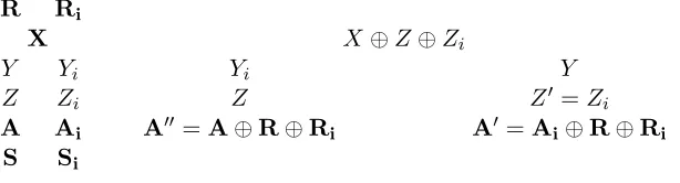
R Ri
X X⊕Z⊕Zi
Y Yi Yi Y
Z Zi Z Z′ =Zi
A Ai A′′=A⊕R⊕Ri A′ =Ai⊕R⊕Ri
S Si
Fig. 6.Random variables involved in the analysis ofChainQuery(X,2) with 3-chains (X, R, S) and (X, Ri, Si).
We now consider a recursive call toChainQuery(Y,3). This recursive call was generated by 3-chain (X, R, S), with (R, S)∈Chain(−1, X,2); this gives Y =F2(X)⊕R. We let {(X, Ri, Si)}
be the set of other 3-chains for Line (F2,−), with (Ri, Si) ∈ Chain(−1, X,2)\ {(R, S)}. For
3-chain (X, R, S), we let:
SkT =P(X⊕F1(R)kR), A=T⊕F6(S)
and for the other 3-chains (X, Ri, Si), we let:
Yi =Ri⊕F2(X), SikTi =P(X⊕F1(Ri)kRi), Ai =Ti⊕F6(Si)
Let also Z =F3(Y)⊕X and Zi =F3(Yi)⊕X. For the ChainQuery(Y,3) call, we consider any
3-chain (Y, Z′
, A′
) such that (Z′
, A′
) ∈Chain(−1, Y,3). SinceChainQuery(Y,3) was recursively called by Line (F2,−), we have thatF3(Y)
$
← {0,1}noccurred; this implies thatX′
=F3(Y)⊕Z′
has the uniform distribution in {0,1}n given H′
. We distinguish two cases:
– Z′
6
=Zi for all i,
– Z′
=Zi for somei.
If Z′ 6= Z
i for all i, then the distribution of Z′ is independent from that of F3(Y) and all
other F3(Yi); since F3(Y) $
← {0,1}n occurred, we have that X′ =F
3(Y)⊕Z′ has the uniform
distribution in{0,1}nand does not belong to the history ofF
2, except with probability at most |F2|/2n; therefore the recursive call toChainQuery(Y,3) is of Type I, except with probability at
most|F4| · |F2| ≤24q3/2n.
IfZ′
=Zi for somei, then we must also show thatX′=F3(Y)⊕Zi does not belong to the
history of F2, except with negligible probability. We have:
X′ =F3(Y)⊕Zi =X⊕Zi⊕Z=F3(Yi)⊕Z
Moreover letting A′ =Y ⊕F
4(Zi), we have: A′
=Y ⊕F4(Zi) =Y ⊕Yi⊕Ai =Ai⊕R⊕Ri
and letting A′′
=Yi⊕F4(Z), we have that:
![Fig. 1. A Merkle-Damg˚ard like construction [9] based on an ideal cipher(right). Messages blocks E (left) to replace a random oracle H mi’s are used as successive keys for the ideal-cipher E](https://thumb-us.123doks.com/thumbv2/123dok_us/1860836.1241785/2.595.92.507.435.555/merkle-construction-messages-replace-random-oracle-successive-cipher.webp)