Wavelet and Curvelet Transform based Image
Fusion Algorithm
Shriniwas T. Budhewar
Dept. of Electronics and Telecomm. Engineering, Government college of Engineering,
Kathora naka, Amravati, Maharashtra, India
Abstract: The prerequisite of more unblemished and realistic Images has contributed the significant development in the Image processing field. An image should encompass every fine aspect of scene, but practically it is impossible to do so due to optical limitations of Image acquiring devices. The solution to this kind of problem is provided by Image fusion Technique. Image fusion can be regarded as the process of merging of two or more images to get a synthetic image. Among the several techniques of image fusion, wavelet transform based algorithm is often practiced. The need for sparse representation and anisotropic way of image decomposition of image for detection of curvature entity, has led the concept of curvelet transform. In this paper, implementation of image fusion algorithm using wavelet and curvelet transform has been described and practical results are compared with several algorithms.
Keywords: Spatial and Transform domain techniques, Wavelet and Curvelet transform, Image fusion, performance metrics.
1. INTRODUCTION
Image acquisition is usually accomplished by a device focusing on particular portion of scene leaving other portion blurred. This happens due to practical limitations of focal depth of devices. For the particular scene, two or more than two images, at different focus plane can be acquired. These images are then merged to form a synthetic image which is known as ‘multifocus image fusion’. Several methods or algorithms of image fusion have been advanced which can be broadly categorized as:[2]
A. Spatial domain based B. Transform domain based
In spatial domain methods, spatial variables i.e. intensity of pixels etc. are considered and manipulation is done with them. The intensity values of pixels are calculated with some mathematical calculations e.g. In maximum select method intensity values of two or more images are compared pertaining to their intensity values and whichever is maximum that is used to assign the intensity of same pixel in the fused image. The point of caution is that the size of input images must be same. This method is simple but does not provide adequate solution as it is just approximation[6]. Second method one can implement by using selecting mean values of pixels. These spatial domain methods have many drawbacks such as reduced contrast, unsolicited artefacts. Another class of fusion techniques seeks out the involvement of mathematical transforms such has wavelet, curvelet. Wavelet transform has been commonly practiced in the field of image processing as it
gives better space-frequency characteristics. Results have revealed the improvement in SNR and spectral resolution over the spatial domain technique. Wavelet function operates on image linearly, but the image is rarely a linear structure [7] [3]
The problem of tracing of curve has led to development of anisotropic, nonlinear transform viz. Curvelet. E. J. Candes and D. L. Donoho proposed Curvelet Transform theory in 2000. It is highly directional transform and is able to trace the curve with minimum coefficient. Curvelet is characterized by three parameters scale, orientation, and translation. The disadvantage of this transform is missing texture and contrast information. Nevertheless applications of curvelet have been up surging widely. Wavelet transform is challenged with representation of edges while curvelet can’t represent texture information clearly. Previous literature shows the implementation of both wavelet and curvelet transform. Theoretically continuous transforms are defined but practically discrete algorithms are implemented by using Matlab viz. discrete wavelet and curvelet transform. [1]
Including first chapter this paper contains five sections; second section deals with wavelet transform whereas curvelet transform has been discussed in third section. Image fusion and results are included in successive sections. Paper is concluded at the end.
2. REVIEW OF WAVELET TRANSFORM
As discussed earlier, the wavelet transform best describes the space-frequency relationship of image. Wavelet transform is composed two sub functions viz. scaling and translation (also called wavelet). In 1-D, continuous wavelet transform can be defined as:[11]
ψψ(τ, s) =
√ x(t).ψ(
τ
) dt (1) Where ‘s’ is scaling parameter and ‘τ’ is translational parameter. ‘ѱ(t)’ is basis function called ‘wavelet function’. The same equation holds true for image as image is two dimensional signal. For better application and ease, discretization of wavelet is preferred so-called ‘Discrete wavelet transform (DWT)’. It can be practically implemented by using Matlab.
∅ ( ) = ∅(2 ) 0 2 1 (2) Where
∅( ) = 1 0 1 0
We can now define a new vector space ‘Wj’as the orthogonal complement of ‘Vj’ in ‘Vj+1’. That is, ‘Wj’ is the space of all functions in ‘Vj+1’ that are orthogonal to all functions in ‘Vj’ under the chosen inner product. Informally, ‘Wj’ contains the details in ‘Vj+1’ that cannot be represented in’Vj’. A collection of linearly independent functions ѱjk(x) spanning ‘Wj’ are called wavelets.
General scaling function of DWT is given by:[9]
ѱ ( ) = ѱ ( ) (3)
There are different functions which can be treated as ‘Mother wavelet’ function, Mother wavelets are orthogonal functions which satisfies ‘Admissibility’ condition. It is given by
1-D multiresolution wavelet decomposition can be forthrightly stretched to two dimensions by introducing separable 2-D scaling and wavelet functions as the tensor products of their 1-D complements. They are given by:
ΦLL=φ(x).φ(y) ѱLH=ѱ(y).φ(x)
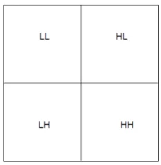
ѰHL=ѱ(x).φ(y) ѱHH=ѱ(x).ѱ(y) For implementation of DWT, ‘Subband coding ’ is preferred and it is straight-forwardly extended for 2D-DWT. Subband coding uses low pass filter (H1) and high pass filter (H0) firstly, subband coding is applied on rows then on columns as shown in fig.1. After first level of decomposition, there will be four frequency bands, namely Low-Low (LL), Low-High (LH), High-Low (HL) and High-High (HH). The next level decomposition is just applied to the LL band of the current decomposition stage, which forms a recursive decomposition procedure. Thus, N-level decomposition will finally have 3N+1 different frequency bands, which include 3N high frequency bands and just one LL frequency band. After the first level the nature of image is shown in fig.2.[9]
Figure 1 Filter bank structure of the DWT Analysis
Figure 2 frequency components after decomposition In above pattern of image, texture information is present in LL function while edge or high frequency information is present in rest of the bands.
For Image reconstruction inverse method of the subband coding is followed. The filter bank structure is shown below in fig.3
2
2
2 HH
LL LH HL
H1 H0
2 H0
H1
2
2 H1
H0
synthesized image
Figure 3 synthesis filter bank for IDWT
In figure 3, upsampling or interpolation is carried out and a pair of low pass (H0) and high pass (H1) filters are used which are same as that of in analysis.
Matlab has provided the instruction for transform and inverse transform. The low pass filtering coefficients are called ‘approximation’ and high pass filtering coefficients are called ‘detail’.
REVIEW OF CURVELET TRANSFORM
E. J. Candes and D. L. Donoho put forth the theory of Curvelet Transform theory in 2000. While dealing with the curve, wavelet transform becomes inefficient as it is linear function and decompose image in a isotropic manner. In this type of decomposition, more wavelet coefficients and more levels of decompositions are needed. Moreover, it requires large amount of time to get fully decomposed image.[10][12]
In curvelet transform, the basis function is in the form of curve i.e. length2~width. It is multiscale transform which operates on image in anisotropic way. Which gives best approximation with less curvelet coefficient in reduced amount of time compared to wavelet transform. The way of approach is shown in fig.4[10]
Figure 4 comparison of wavelet and curvelet transform Curvelet functions are characterized by scale, orientation and translational parameters, values of which are adaptably defined. The curvelet transform has four stages:[10]
I. Sub-band decomposition:
In this step, the image is divided into individual subband frequencies. Mathematically, it is given by:
f α (P0f, ∆1f,∆2f, K) (4) where ‘f’ is image matrix or function, ‘P0’is low pass filter, ∆1,∆2,... are band pass filters.
II. Smooth partitioning:
A grid of dyadic squares is defined:
( )
[
] [
]
sk k k k k k
s s s s s
Q
,1, 2=
21,
12+1×
22,
22+1∈
Q
(5) Qs – all the dyadic squares of the grid.
Let w be a smooth windowing function with ‘main’ support of size 2-s×2-s. For each
square,‘wQ’ is a displacement of w localized near
Q. Multiplying Δsf with wQ (∀Q∈Qs) produces a
smooth dissection of the function into ‘squares’. The windowing function w is a nonnegative smooth function.
III. Renormalization:
Renormalization is centering each dyadic square to the unit square [0,1]×[0,1]. For each Q, the operator TQ is defined as:
( )
T f(
x1,x2)
2 f(
2 x1 k1,2 x2 k2)
s s
s
Q = − − (6)
IV. The Ridgelet Transform:
Ridgelet are an orthonormal set {ρλ} for L2(ℜ2) which
divides the frequency domain to dyadic coronae |ξ|∈[2s,
2s+1]. In the angular direction, samples the s-th corona at least 2s times. It is shown in fig.5
Figure 5 Ridgelet function
Curvelet transform can be implemented by the frequency wrapping algorithm given by E. J. Candes and D. L. Donoho. It is available at http://www.curvelet.org.[1]
3 IMAGE FUSION
The transform based methods follow a generic method which is shown in fig 6
Figure 6 generic method of transform based fusion
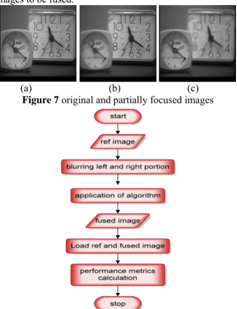
Transformation is applied on images to be fused to transform them into frequency or space-frequency domain. The coefficients obtained during this process are used for the fusion. Fusion rule is nothing but the criteria for the selection or impositions of the coefficients of fused image, e.g. maximum coefficient selection, minimum coefficient selection etc. after fusion reverse transformation is applied to get image back into spatial domain. The algorithm for the image fusion is given in fig.8. for the experimentation the raw images are derived from single image, by blurring either left or right side of image. Left blurred image can be treated as right focused image and vice versa. These two images can be fused and the results can be validated by comparing it with original image.
For the fusion, the selected image is shown in fig.7 (a). the right and left focused images which are obtained by blurring the part of image are shown in fig (b) and (c) respectively. Note that in fig (b),larger, square alarm clock is clearly visible while in fig (c) smaller, round clock is clearly visible. These two images form the set of images to be fused.
(a) (b) (c) Figure 7 original and partially focused images
Figure 8 Image fusion algorithm
1
2
-s4 RESULTS
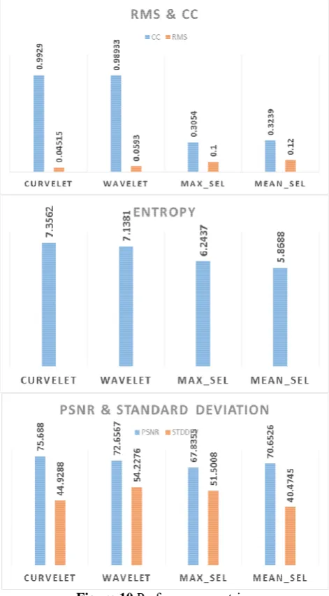
For above shown images, fusion is carried out by using both the transforms and the resulting images are compared. For validation of the results statistical parameters are taken into account. Five performance metrics are calculated for the original, and fused images which are shown in fig. 9, viz. PSNR, standard deviation, cross correlation, Entropy.[4][8]
Curvelet fused image Wavelet fused image Figure 9 Transform based fusion Five performance metrics are detailed below:
I. Peak signal to noise ratio (PSNR):
Peak signal to noise ratio is defined as ‘ratio between the maximum possible power of a signal and the power of corrupting noise that affects the fidelity of it’s representation’.
2
10 10
( 1) 1
10 log L 20 log L
PSNR
MSE RMSE
− −
= =
(7)
Where ‘L’ is maximum intensity level possible.
II. Standard deviation:
Standard deviation is a measure of contrast in an image.larger is standard deviation, the higher is contrast.
( ) ( )
(
( ))
1 1 2
1
2 0 0
2 0
,
N M L
i j
k k
k
A i j m
r m p r
NM
σ σ
− − −
= = =
−
= =
− =
(8)
III. Entropy: Measure of information present in the image.
= ∑ ( ). log ( ) (9)
IV Root mean square error:
Root mean squared error is the measure of differences between the reference images and fused image.
( ) ( )
(
)
1 1 2
0 0 1
, ,
N M
i j
RMSE MSE A i j B i j NM
− −
= =
= =
−(10)
V Cross correlation:
Cross correlation is used to find out the similarities between fused image and registered image.
For the fused image the above parameters are calculated and same is done with spatial domain techniques shown in graph. Based on the values the graphs are drawn which are shown in fig. 10
Figure 10 Performance metrics
5. CONCLUSION
Note that all the parameters except RMS are higher for transform based methods. Moreover from the graph it is clear that transform domain methods prove to be efficient over the spatial domain methods. Less value of RMS for the transform domain methods clearly indicates that the fused image is void of artefacts. Higher value of PSNR shows that image is less prone to noise compared to spatial domain methods. Entropy is approximately same for all the methods. Cross correlation coefficient value approximates to 1, which represents the degree of similarity to that of original image.
that curvelet transform can represent the curves efficiently than wavelet transform and wavelet has better capability to represent texture, contrast information than curvelet.
From above discussion it is clear that transform domain methods proved to be efficient over spatial domain methods. In spite of certain disadvantages for transform based methods as explained earlier, they are popularly used in the field of image processing. One can use two or more transform to counter correct the limitations of transform[12].
REFERENCES
[1] CurveLab, [Online]. Available: http://www.curvelet.org.
[2] K. Shivsubramani, K. P. Soman, "Implementation and Comparative Study of Image Fusion Algorithms," International Journal of Computer Applications, vol. 9, no. 2, p. (0975 – 8887), Nov 2010. [3] Mathworks corporation, "Matlab and Simulink,"
[Online].Available:
http://www.mathworks.in/matlabcentral/answers/.
[4] M. Deshmukh and U. Bhosale, "Image Fusion and Image Quality Assessment of Fused Images," International Journal of Image Processing (IJIP), vol. 4, no. 5.
[5] A. Saha , G. Bhatnagar and J. W. Q. M., "Mutual spectral residual approach for multifocus image fusion," Digital Signal Processing, ELSEVIER, vol. 23, p. 1121–1135, March 2013.
[6] D. k. Sahu and M. P. Parsai, "Different Image Fusion Techniques – A Critical Review," International Journal of Modern Engineering Research, vol. 2, no. 5, pp. 4298-4301, sep-oct 2012.
[7] R. Sharma and K. Rani, "Study of Different Image fusion Algorithm," International Journal of Emerging Technology and Advanced Engineering, vol. 3, no. 5, 2013.
[8] M. A. P. A. Dr.S.S.Bedi, "Image Fusion Techniques and Quality Assessment Parameters for Clinical Diagnosis: A Review,"
International Journal of Advanced Research in Computer and Communication Engineering, vol. 2, no. 2, pp. 2319-5940, Feb 2013.
[9] R. C. Gonzalez and R. E. Woods, "Wavelets and Multiresolution processing," in Digital Image Processing, New Jersey, Prentice Hall, 2002, pp. 350-386.
[10] Jianwei Ma and . G. Plonka, "The Curvelet Transform : A review of recent applications," in IEEE SIGNAL PROCESSING MAGAZINE, 2010.
[11] R. Polikar, "The Wavelet Tutorial by Robi Polikar," 2001.[Online].Available:
http://users.rowan.edu/~polikar/WAVELETS/WTpart1.html. [12] B. Y. Shutao Li, "Multifocus image fusion by combining curvelet
and wavelet transform," Pattern Recognition Letters, ELSEVIER,
no. 28, p. 1295–1301, 2008. D. Hall and J. Llinas, "An introduction to multisensor data fusion", Proceedings IEEE, Vol. 85(1), pp. 6-23, 1997
AUTHOR
Shriniwas Budhewar received the B.E. in Electronics and Telecomm. Engineering from Pad. Dr. D. Y. Patil Institute of Engineering and Technology, Pimpri, Pune in 2011. Presently, he is pursuing his M-Tech. in Electronic system and Communication from Govt. college of Engineering, Amravati. His area of interest includes Digital Image and signal processing, mathematical transforms. Recently he is working on the project ‘Curvelet and wavelet transform based image fusion.’