ABSTRACT
Kaszycki, Gregory J.. An Adaptive Non–Parametric Kernel Method for
Classi-fication (Under the direction of Dr. Dennis R. Bahler.)
One statistical method of estimating an underlying distribution
from a set of samples is the non–parametric kernel method. This method can
be used in classification to estimate the underlying distributions of the various
classes. Since it can be shown that there is no perfect shape to a kernel function
used to estimate an underlying distribution, several functions have been
pro-posed and none is superior in all cases. This thesis demonstrates that a function
can be created that adapts its shape to fit the properties of the underlying data
set. The function adapts its shape based on a pair of parameters and the
algo-rithm uses a hill–climbing algoalgo-rithm to determine the best pair of parameters
to use for the data set. This method gets consistently better accuracy than
exist-ing non–parametric kernel methods and comparable accuracy to other
classifi-cation techniques.
An Adaptive Non–parametric Kernel
Method for Classification
by
Gregory J. Kaszycki
A Thesis submitted to the Graduate Faculty of
North Carolina State University
in partial fulfillment of the requirements
for the Degree of
Doctor of Philosophy
Computer Science
Raleigh
2000
ii
BIOGRAPHY
iv
ACKNOWLEDGEMENTS
I appreciate the help and encouragement from all of my committee members:
Dr Dennis Bahler, my advisor, has helped me get through the field and the
jargon with effective guidance and patience. He has also allowed me to
pur-sue the areas that interested me and still kept me focused on an attainable
objective. Dr David Dickey has been a great resource on the statistical end
of things. Dr Matthias Stallmann has given me good advice on a broad
range of issues and been concientious about his and my academic
responsi-bilities. Dr James Lester gave me my introduction to AI and has always
been enthusiastic about my efforts.
My Wife Lisa: Going back to school at this stage was not the easy thing to do,
but you understood that it was what I wanted to do and you made it possible.
Dr Carol Wellington: Thanks for helping me believe that I could do this.
Dr Vicki Jones: Your interest and enthusiasm about my work has made it easier
to focus when the tedium slowed me down.
Contents
*34 /' *(52&3 6*** *34 /' "#,&3 *8
"%# %#!&%!
,"33*'*$"4*/. 24*'*$*", .4&,,*(&.$& 63 4"4*34*$3 "2"-&42*$ 63 /.0"2"-&42*$
2(".*:"4*/.", 6&26*&7
"%# #% % %!$ ! #
&$*3*/. 2&&3 &$*3*/. 2&& &4)/%/,/(9 0,*44*.( 2*4&2*" *-*4"4*/.3 /' &$*3*/. 2&&3
#,*6*/53 &"%.$& &$*3*/. 2"0)3 3 5,4*6"2*"4& &$*3*/. 2&&3 *.&"2 "$)*.&3 &&%'/27"2% &52", &43 6&26*&7 /' &&%'/27"2% &52", &43 "$+02/0"("4*/. *. &&%'/27"2% &43
2"*.*.( *-&
/.$&04 *-*4"4*/.3 &4)/%3 /4 %%2&33&% "9&3*". &43
&(2&33*/. 2&&3 .%5$4*6& /(*$ 2/(2"--*.( 5--"29 /' &4)/%3
"%# %%$% %!$ ! $$%!
*2&$4 /%&, &4)/%3 /' 4"4*34*$", ,"33*'*$"4*/. /(*34*$ &(2&33*/.
)& 2/#*4 /%&, '/2 *."29 54$/-&3 ,"33*'*$"4*/. #9 34*-"4*/. "2"-&42*$ &4)/%3 /' 34*-"4*/. /."2"-&42*$ &4)/%3 /' 34*-"4*/. &(2&33*/. 0,*.&3 5--"29 /' 4"4*34*$", ,"33*'*$"4*/. &$).*15&3
"%# "%' ! #%# %! ! $$%!
vi
"%# ("# % $
/-0"1*2/. /' $$41"$8 /-0"1*.( 3/ /3)&1 ./.0"1"-&31*$ +&1.&, '4.$3*/.2 /-0"1*.( 3/ &$*2*/. 1&&2 /-0"1*.( 3/ &41", &32 /-0"1*.( 143&'/1$& 2&"1$) 3/ *,,$,*-#*.( ,(/1*3)- ".",82*2 /' 3)& %"03*5& &1.&, 4.$3*/. &3)/% &"241*.( $34", 14.3*-&2 /' 3)& %"03*5& &1.&, 4.$3*/. &3)/% &,"3*/.2)*0 /' 03*-", 1 , 3/ "3" &3 )"1"$3&1*23*$2
"%# # !# $% #
*,,$,*-#*.(
)& 11&(4,"1 41'"$& 1/#,&- *. *,,$,*-#*.( ..&",*.( /-&.34- ".%/- 4-02 /,43*/. !2&% '/1 )*2 &"1$)
"%# ("# % $&%$
/-0"1*2/. /' $$41"$8 6*3) 7*23*.( /.0"1"-&31*$ &1.&, &3)/%2 $$41"$8 /' 3)& "%"03*5& -&3)/% 52 &7*23*.( ./.0"1"-&31*$ +&1.&, -&3)/%2
03*-", )"0& /' 3)& %"03*5& &1.&, 4.$3*/.
/-0"1*2/. /' $$41"$8 6*3) /-0"1*2/. /' $$41"$8 6*3) &&%/16"1% &41", &3 &,"3*/.2)*0 /' 1 , 3/ "3" &3 )"1"$3&1*23*$2 1 52 /*2& , 52 /-0,&7*38 4..*.( *-&2
"%# ! &$! $
$$41"$8 !3*,*38 %%*3*/.", &2&"1$) 1&"2
,(/1*3)- -01/5&-&.3
*.&"1 &(1&22*/. &,"7*.( 3)& $/.231"*.32 /. 3)& %"3" 2&32 "3)&-"3*$", /4.%"3*/.2
"%# !#") "" ( ' %
viii
List of Figures
1/<9- "1473- -+1:165 #9-- 1/<9- "1473- -+1:165 #9-- 65 ;0- $51; "8<)9-
1/<9- 1:+9-;1A-, 15-)9 <5+;165 1/<9- 6/1+)3 .<5+;165 15 ' )5, ( 1/<9- -+1:165 #9-- .69 "1473- 6/1+)3 <5+;165 15 ' )5, ( 1/<9- -+1:165 9)70 .69 "1473- 6/1+)3 <5+;165 15 ' )5, (
1/<9- *31=16<: !-),5+- -+1:165 9)70 .69 "1473- 6/1+)3 <5+;165 15 ' )5, (
1/<9- 15-)9 )+015- >1;0 #09-- 3)::-: 1/<9- 9;1.1+1)3 -<965 1/<9- ")473- -9+-7;965 !-:765:- <5+;165 1/<9- 3)@-9 5-<9)3 5-;>692 1/<9- 6/1:;1+ !-/9-::165 <5+;165 1/<9- )9)4-;91+ 3):: )7715/ 66, ?)473- 1/<9- )9)4-;91+ 3):: )7715/ ), ?)473- 1/<9- )9)4-;91+ 3):: )7715/ 5+699-+; :;14);- 6. ;0- ), ?)473-
1/<9- $51.694 657)9)4-;91+ <5+;165 15 5- 14-5:165 6; 56</0 "466;015/
1/<9- $51.694 657)9)4-;91+ <5+;165 15 5- 14-5:165 #66 <+0 "466;015/
1/<9- $51.694 657)9)4-;91+ <5+;165 15 65- 14-5:165 6,-9);- "466;015/
1/<9- 6<9 5657)9)4-;91+ 2-95-3 <5+;165: $:-, *@ "" >1;0 9 5694)3 9
1/<9- )3+<3);-, -+)@ <5+;165 15 5- 14-5:165 >1;0 %)9@15/ -=-3: 6. $51.694 61:- 15 '
1/<9- ,)7;1=- 657)9)4-;91+ <5+;165 >1;0 %)9@15/ 3 )5, 9 1/<9- ,)7;1=- 657)9)4-;91+ <5+;165 >1;0 %)9@15/ 3 )5, 9 1/<9- ,)7;1=- 657)9)4-;91+ <5+;165 >1;0 %)9@15/ 3 )5, 9 1/<9- 19+3- 9;1.1+1)3 );) "-; 1/<9- 3317:- 9;1.1+1)3 );) "-;
1/<9- 6? 9;1.1+1)3 );) "-; 1/<9- <33:-@- 9;1.1+1)3 );) "-; 1/<9- ++<9)+@ ): ) .<5+;165 6. 9 3 .69 ;0- <33:-@- );) "-; 1/<9- ++<9)+@ =: ! 3 .69 ;0- 1=-9 );) "-;
List of Tables
)# !!1.!5 ,$ .*#0.'! 1#// ,+ " 4*-)# )# &.!0#.'/0'!/ ,$ 0&# 0 #0/ /#" '+ 0&# #/0/ )# !!1.!5 ,$ .10# ,.!# #.!& 2/ '))!)'* '+% )# #.$,.*+!# ,$ 4'/0'+% ,+-.*#0.'! #0&,"/
)# ,*-.'/,+ ,$ 0&# "-0'2# #0&," 0, #/0 4'/0'+% ,+.*#0.'! #0&,"/
)# ,*-.'/,+ ,$ 0&# "-0'2# #0&," 0, 0&# ,.*) 1+!0',+ )# ,*-.'/,+ ,$ 0&# "-0'2# #0&," 0, 0&# -+#!&+'(,2 1+!0',+ )# ,*-.'/,+ ,$ 0&# "-0'2# #0&," 0, 0&# '3#'%&0 1+!0',+ )# ,*-.'/,+ ,$ 0&# "-0'2# #0&," 0, 0&# .'3#'%&0 1+!0',+
)# ,*-.'/,+ ,$ 0&# "-0'2# #0&," 0, 4'/0'+% ,+.*#0.'! #0&,"/ 0,0)/
)# -0'*) .*#0#./
x
NOTATION
The information for this dissertation was taken from several different sources without a common notation. In order to be consistent, a single notation was used throughout this dissertation. This notation may not be consistent with the notation of the source from which the information was gotten, but it will be consistent throughout this dissertation. This section describes that notation.
A = the number of attributes a = a specific attribute
|a| or V = the range of an attribute
C = a clause in predicate logic or prolog
c = a concept (a mapping of points to a class)
e = the difference between the response y and the actual class r
f or g = a general function
H = the set of possible hypotheses
h = a hypothesis that tries to represent the concept
h’ = a program that represents a hypothesis
K = the number of classes in the data set k = a specific class
k’ = an encoding for a class k
l or p = a literal from a clause
N = the number of examples of data in the set N(k) = the number of examples from class k
N(k) = the expected number of examples from class k r = a range or smoothing parameter for kernel functions v = the value of an attribute
W = a weight space of of a learning method w = a specific set of weights
X = the set of data examples or a complete vector of an example x = a specific data example
Y = a response variable
y’ = an encoding of a response
= a vector of coefficients for a linear combination
= a learning rate
= the mean of a function
= a set of parameters to specify an application of a parametric family
= standard deviation
1
Chapter
1.
Introduction
In both Artificial Intelligence (AI) and in statistics, a common problem is that of
clas-sification. Sometimes referred to as inductive reasoning or machine learning or pat-tern recognition, the goal is to classify an example which has not been seen before and
for which the true classification is not known, based on data from previous examples [16].
There are certain techniques that are classically viewed to be AI techniques and cer-tain techniques that historically belong in the realm of statistics, but both sets of tech-niques aim at doing the same task. Furthermore, there are small general differences in the goal, in how the problem is viewed and how the problem is treated, but these dif-ferences are not hard and fast rules. The lines are blurry and the distinctions are based more on history and convention.
The different techniques for classification, in both statistics and AI, have trade–offs in terms of accuracy, representational limitations and speed (both in initial learning and in processing complexity for new examples). Additionally, these different techniques make different assumptions about the general form of the problem and its solution. These differences and the limitations of these methods will be explored and a new method will be introduced that is a variation of an existing statistical technique called
non–parametric kernel functions. This new technique is an “adaptive”
non–paramet-ric kernel method (ANPK).
1.1 Classification
do this by looking for common patterns as with decision trees and inductive logic pro-gramming (ILP) or with numeric formulae, as with logistic regression or parametric kernel functions.
The information about an example is usually a set of numeric measurements called
attributes or features (such as the height of a person). But the attributes can also be an
ordinal classification (like short, medium and tall) or a nominal variable (like color). These attributes are usually the same for all of the examples, but there can be missing data.
The target classification is from a finite set of classes (like weather types). For gen-erality, it can be viewed as a binary classification since a multi–class problem can be viewed as a set of binary classification problems (like rainy vs not rainy, clear vs over-cast, chilly vs mild...) The classifier just has to make sure that for a new example it chooses one and only one class.
1.2 Artificial Intelligence vs Statistics
There are three areas of difference between AI methods of classification and statistical prediction methods. Primarily, AI methods usually try to retain some artifact of the information in the examples. Part of the goal is to provide a “learned” representation of the concept that provides some insight about the concept. A concept is a mapping from the attribute space to the classifications [8,53]. The attribute space is an A–di-mensional space made up of the cross products of each of the domains of the attrib-utes.
Ideally this “concept” will provide some insight into the relationship between the at-tributes and the classification. Also, this concept can be stored independently from the original data set. In statistics, the classification is usually based on formulae that give little or no human insight into the relationship without expert analysis.
This difference has exceptions. Neural nets (in AI) do not provide human readable insight into the concept, while logistic regression does give information about the key factors.
A second difference is the way that the problem is viewed. The example can be
un-3
derlying borders of these regions are viewed to be arbitrarily complex, but a specific region is generally assumed to belong to one class only. Overlapping distributions are viewed as conflicting data. Decision trees and neural networks will “over–fit” the data unless specific actions are taken to stop them. This over–fitting leads to learned concepts that are very complex and that “guess” correctly for all of the training exam-ples, but do not generalize well to new examples.
The AI concept is viewed as a set of regions. A region of the attribute space is a set of contiguous points in the attribute space in which all points within a small distance are of the same class. These regions can be represented by their borders rather than hav-ing the points enumerated. In fact, the points in these regions cannot be enumerated because their domains are numeric and continuous.
More recent techniques in fuzzy logic are trying to move away from this view towards a more overlapping view [6,63], but the basic mapping of regions to classifications is still the goal.
For most problems, the statistical paradigm may seem more intuitively correct. Ex-amples from more than one classification may be present in a single area. However, the point that is measured in class k is most likely (by definition) to come from the class that has the highest frequency at that point. The difficulty is deciding when changes in example frequency are due to random sampling of two PDFs and when it signals a significant change in the predominant classification.
The third difference is that learning systems in the machine learning community has been largely empirical rather than theoretically motivated [16]. The statistical re-search tends to be more theoretically grounded [30]. For example, in parametric ker-nel functions and logistic regression, variances and statistical significance can be put on the parameters of the classification formulae. There is generally not such informa-tion for the thresholds in a decision tree or the weights of a neural network.
This additional theoretical foundation is due in part to the fact that statistics is a much more mature discipline.
1.3 Parametric vs Non–parametric
dis-tributions of the different classifications are multivariate normal or from some other well–known distribution. It may be assumed that the points of a given class are all part of a single convex cluster and that all of the points of that class are within some small distance of one another.
Non–parametric methods are usually computationally more intense because they make no assumptions about the underlying distribution and take each point as contributing its own information to the overall concept solution.
Decision trees are a parametric method as are statistical parametric methods and meth-ods based on a model form. Neural nets and non–parametric additive kernel methmeth-ods are examples of non–parametric methods.
1.4 Organizational Overview
The remainder of this thesis is organized as follows. Chapter 2 describes general clas-sification methods in artificial intelligence. Chapter 3 describes general clasclas-sification methods in statistics. This is to give a general background in current methods and to show how the new method fits into the classification arena. Chapter 4 describes the new approach (Adaptive non–parametric kernel function – ANPK) that is a variant of a statistical method described in Chapter 3, and Chapter 5 discusses how that method was evaluated in comparison to the common methods introduced in Chapters 2 and 3. Chapter 6 gives a discussion of what kind of information can be gleaned from the re-sults of this method. Chapter 7 gives the empirical rere-sults of the experiments run on this method and general overall conclusions are in Chapter 8.
5
Chapter
2.
Artificial Intelligence
Methods of Machine
Learning
The basic paradigm of classification for the different AI methods is the same as it is for classification techniques in statistics. The program is given a set of examples for which a classification is known. An example consists of a set of values for some set of attributes and the classification category into which the example falls. The method tries to determine the correct mapping of attribute values to the target classification. Then given a new example, for which the target classification is not known, the pro-gram tries to predict the target classification [51,67].
When the classifier has “learned” the concept, it can input new examples and produce a classification output. The classification method has some structure, formula, or con-cept representation whose parameters must be adjusted to create a mapping of the ex-ample space to the classifications [67]. The goal is to make this mapping accurate for the training examples and also for new examples for which the correct classification is not already known.
An important goal of machine learning techniques in AI is not only to achieve high accuracy, but to derive a learned concept from the data. A concept is a mapping of some set of points in the example space to a classification [8,53]. Ideally, this concept will yield insight into the classification problem.
Each of the attributes in the examples has a domain and the Cartesian product of these domains makes up an A–dimensional space. Each of the A attributes is an axis in this A–dimensional space and each example is a point in that space.
The “true” concept is a mapping of points in this space to each concept. The known data points are hopefully accurate examples of this mapping. The goal of machine
learning is to come up with a concept representation that accurately reflects the “true”
con-cept space) and H (the hypothesis space), and the problem is to find, for each c ∈ C, some h ∈ H which is a good approximation to c.” [8]
In the “real” concept, these regions may be of arbitrary shape and a single concept may have an arbitrary number of these regions. The “real” concept may be an enu-merated list and have no defined regions at all. In general, classification methods do not consider enumerated lists as concepts that can be learned because they do not gen-eralize outside the training set.
A concept is complete with respect to a set of examples if it entails all of the positive examples. That is, all of the positive examples will be guessed as positive examples by the classifier. It is consistent if it does not entail any of the negative examples. That is, none of the negative examples would be classified as positive.
The machine learning program must create a learned concept that contains as many of the real concept points as it can without including points that are not part of the real concept. It must do this within the representational limitations of that particular ma-chine learning technique.
The different machine learning techniques have different ways of representing these
concepts and therefore different representational limitations in what concepts they can
represent well and learn well. These limitations create assumptions that the true con-cept mapping can fit the form of these limitations.
Some assumptions that most machine learning techniques make is that the underlying concept is a relatively simple mapping or that it can be approximated with a simple hypothesis space. These assumptions can be explicit or simply a built–in part of the technique. Since the learning methods do not typically represent concepts as enumer-ated lists, they assume that the points of the target concept can be approximenumer-ated with some description of a region or set of regions, that the regions are generally concave, that there are not a large number of disjoint regions and that the technique being used can derive a concept description that “reasonably approximates” the real or underlying concept.
Since any machine learning technique has some limitations in both its representational methods and its methodological assumptions, the creation of this concept may lose some information from the original data. The goal is to make this derived concept a reasonable generalization of the data.
7
The major inductive techniques that this chapter will address include Decision Trees and feed–forward Neural Nets. Decision tree programs include C45 and ID3 [56]. The most common Neural Nets are feed–forward nets that use back–propagation to adjust the weights. (The software program used in these experiments to simulate the behavior of the neural net was Enterprise Miner from SAS.) These different AI techniques have advantages and disadvantages over each other in terms of computa-tion time and understandability, but beyond that are representacomputa-tional limitacomputa-tions that dictate what kind of solutions they can represent or learn well.
2.1 Decision Trees
A simple example decision tree for weather prediction (taken from Quinlan [56]) might be:
Outlook
Humidity Windy
sunny rain
overcast
high normal
true false
N P
P
N P
Figure 1: Simple Decision Tree
2.1.1 Decision Tree Methodology
9
also stop if the examples at a given node has a large majority of one class. This avoids over–fitting [56].
In general, a node can have a different branch for each value that the attribute can take on, but many tree algorithms are limited to binary decisions. Attributes with more than two outcomes can be translated into binary outcomes so there is not really a limi-tation, but it does affect the splitting choice. Most of the splitting criteria measures will favor multi–valued attributes over binary outcomes [52].
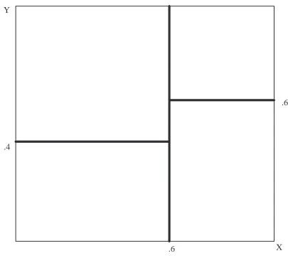
In the A–dimensional attribute space, the threshold at a node creates an (A–1) dimen-sional hyperplane that is orthogonal to the splitting axis and splits the A–dimendimen-sional space into two sub–regions.
In Figure 2, a simple example of these perpendicular hyperplanes shows the first threshold breaks the unit square into x<.6 and x>.6. For the region where x<.6, the next threshold breaks the region into y<.4 and y>.4. For the region where x>.6, the next threshold breaks the region into y<.6 and y>.6. This corresponds to a simple binary decision tree with a depth of 2.
For a nominal value, the space is discrete and the new node splits it into those exam-ples that have a particular nominal value for an attribute and those that don’t. If the algorithm allows for multiple values of the decision attribute, then each path is one “slice” of the remaining space. If it only has binary nodes, then the branch that con-tains the value is a single slice of the attribute space.
Y
.6 .4
.6
X
11
2.1.2 Splitting Criteria
The goal of a decision tree learning algorithm is to break the attribute space into gions that are dominated by a single class. When the learning is complete, these re-gions are represented by the leaf nodes of the tree and will represent classifications. The accuracy of these classifications will be higher if these leaf–node regions are ho-mogenous with respect to the known examples and if they are a representative set, then the regions will be more homogeneous with respect to the “real” concept.
Decision tree algorithms are greedy algorithms that choose the attribute that splits the data best at the current node. They are greedy in the sense that they do not have a global strategy, but choose a split based only on the data at this current node. Differ-ent algorithms may use differDiffer-ent criteria, but they are all trying to get the split that creates the most homogeneous regions with respect to the examples and their classes. [52,67]. While these different criteria may have different performance results on some data sets, their advantages and disadvantages are not consistent [52,67] The dif-ferences in the methods are simply how they measure “purity”.
One common method used in ID3 [56] uses information gain as the criterion to judge the purity of a split. ASSISTANT was a modification of ID3 that included unre-stricted integers and C4.5 was an additional improvement to include real–valued at-tributes. The information function (I) is based on the expected amount of information (number of bits) needed to communicate a message:
where is the number of examples in the class k, is the number of examples that are not in class k (negative examples) and N is the total number of examples. As an example, suppose we have 16 examples and 8 are positive and 8 are negative. The information needed to differentiate the example is:
The expected amount of information needed after a split is the weighted average of the
I functions for the sub–trees. When splitting on an attribute, the examples will be split
into the different sub–trees based on the value of the splitting attribute. The I function for each of these new splits is calculated and multiplied by the percentage of examples that have that attribute value (the percentage that would go to that node).
This is the weighted sum of the information in the various sub–trees of this node where aj is attribute j and Vi is the number of different values that attribute j can take on.
Suppose from the example there are two attributes to split on. One attribute splits the 16 examples into two groups of 8 where one group has 5 positive and 3 negative ex-amples and the other group has 3 positive and 5 negative exex-amples. The expected in-formation in the sub–tree is:
Suppose the other attribute splits it into one group of 6 positive and 1 negative and the other group of 2 positive and 7 negative. The expected information is:
The information gain for a node is the amount of information needed to convey this message minus the amount of information in the remainder of the tree. The informa-tion gain funcinforma-tion g is the amount of informainforma-tion at this node minus the expected val-ue of the information at the sub–trees: . For the first attribute it is 1 – .954 = .046 and for the second attribute it is 1 – .689 = .311. There-fore the second splitting attribute has a better information gain than the first.
Since the amount of bits needed to communicate a message is highest when the pos-sible messages are equally likely, this criterion is best when the attribute splits the ex-amples into the subsets that are most heavily one class or another. Clearly, the second attribute splits the examples more purely than the first attribute and the information gain reflects that. The best splitting attribute would split the examples into all of the examples of one class in one subset and all of the examples of the other class in the other subset. This split would be most pure and have the highest information gain. Probabilistic criteria, like chi–squared tests, can also be used [52]. The chi–squared statistic measures the departure from expected values for the splitting criterion.
where is the expected number of class j for value i of this attribute and
is the actual number of class j with value i. When the examples at the attribute
13
measures that split the remaining examples in ways that are most pure. While a spe-cific statistic may outperform another on a spespe-cific data set, it has not been shown that any one statistic is universally better for accuracy [52].
Martin [49] gives a statistical criterion that yields the probability that the given split would occur with an attribute that was independent of the outcome. With this criteri-on, not only could the choice of attribute be made, but the stopping criterion could be set up so that if no remaining attribute was “significant” at some level of confidence, the tree induction could be stopped. This keeps the tree from growing and having to be pruned later.
When an example reaches the leaf node of the tree, it is normally classified into the majority class at that leaf. However, if the leaf is close to evenly split, the classifica-tion may be left undetermined or a regression model may be made of the examples at the leaf node [28].
2.1.3 Limitations of Decision Trees
Whichever splitting criteria are used, the top–down induction of decision trees (TDIDT) is a greedy algorithm and deals only with the best split at the current node without any global strategy. A global strategy using dynamic tree restructuring has been introduced, but these are heuristic searches [20,64]. The entire tree space is com-putationally infeasible to search completely [20].
Regardless of how the tree is induced or learned, the splits at the nodes represent A–1 dimensional hyperplanes that are orthogonal to the axis of the splitting attribute [14]. Since the splitting nodes all create these perpendicular planes, the system cannot rep-resent concepts that contain sloped or curved surfaces or boundaries. (These bound-aries would represent functions of multiple attributes.) The decision tree can
approximate them with many branching points, but this creates its own problems. The amount of space used by the tree is exponential in the depth of the tree. Each new split creates another level of the tree.
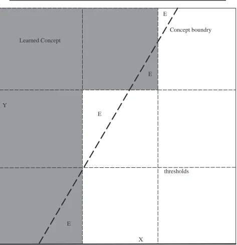
For example, suppose we were trying to solve a concept whose true boundary was a line in the xy plane. But suppose that x and y have been thresholded into small, me-dium and large regions as seen in Figure 3.
The regions labelled with the E’s represent regions for which there are errors because the error region is indistinguishable from the rest of the block by the net since they have the same inputs.
.25 times the volume of all multi–dimensional pixels that fall on the border of the re-gion. (The minority classification would be uniformly distributed between 0 and 50 percent of the box.) So error is introduced by the act of thresholding and partitioning.
E
E
E E
X Y
Concept boundry Learned Concept
thresholds
15
Cochran and Hopkins [21] address the effects of descretizing variables in a single di-mension, but in the multivariate classification problem it is not well understood. It depends on the shape of the actual region being approximated, the number of tree lev-els and the probability density function of the examples in the attribute space.
2.1.4 Oblivious Read–Once Decision Graphs (OODGs)
One of the problems of basic decision trees is that the number of nodes in the tree is exponential in the number of attributes (the depth of the tree). This can create storage and readability problems for the representations of the trees. Variations on the basic tree structure can reduce this storage size [43].
1 2 x 1
2 y
1 2 X
Figure 4: Logical function in X and Y
For the function:
17
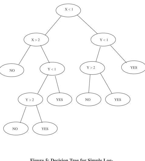
X < 1
X > 2 Y < 1
Y < 1 Y > 2
Y > 2 NO
NO
NO
YES
YES YES
YES
while a decision graph could reduce the number of interior nodes from 7 to 4 and the number of leaf nodes from 6 to 4. (Figure 6). The duplicate sub–tree has been elimi-nated.
X < 1
X > 2 Y < 1
Y > 2 NO
NO YES
YES T
F
F
T
F T
T F
19
A read–once decision graph (Figure 7) is one in which for any path through the graph, no attribute will be seen more than once. It further reduces the size of the graph from 4 interior nodes and 4 leaf nodes to 2 interior nodes and 3 leaf nodes.
X
Y
NO
NO
YES < 1
> 2
< 1
> 2
other
other
Figure 7: Oblivious Read–Once Decision
Graph for Simple Logical Function in X
and Y
21
In experimental testing, the OODG algorithm out–performed traditional tree algo-rithms on artificial data sets (in terms of accuracy) but performed worse on natural data sets. [43]. No data was given for storage use, but the implication is that it would take as much or more storage to “learn” the structure but would use less once the structure was complete.
OODGs compress the number of nodes in the tree (or graph), but they don’t change the nature of the decisions and so the representational limitations of them are the same as for basic decision trees.
2.1.5 Multivariate Decision Trees
Brodley and Utgoff [14] discuss variations on univariate decision trees that use linear combinations of the attribute values. These combinations of attributes can take the form of Multivariate Decision Trees, where each node is a linear threshold unit (LTU) or the combinations can take the form of a linear machine (LM).
A LTU is a binary test of the form WTX≥0, where W is a weight vector and X is the instance vector. This allows a branching on a linear combination of more than one at-tribute.
Conceptually, this linear threshold creates a hyperplane that is not orthogonal to an axis, but there is only one hyperplane for a single binary decision. However, a tree could contain additional multivariate tests to split and avoid the representational limi-tation of always having the hyperplanes orthogonal to an axis.
In practice, these do not get used vary much because one of the major benefits of a de-cision tree is that it is easy to understand and the multivariate combinations tend to lose that property [14]
This method also creates special problems with respect to nominal attributes with more than one possible value that are not ordered. Whenever numeric formulae are used on nominal variables, the multiple values are translated into numbers and the lin-ear combination will create an automatic ordering and create bias. One possible solu-tion is to create a set of binary attributes that are true if and only if the multi–valued nominal attribute is equal to a particular value.
The goal of choosing the coefficients may be to maximize a partition–merit criteria or to maximize the purity of split [14]. Whatever the goal, the method is recursive like the single–variable decision tree and heuristic because choosing the attributes is NP complete and the coefficient space is infinite [14]
The weights of one iteration are based on the error in the results of the previous itera-tion times the learning rate .
W is the weight vector, X is the instance vector and y is the actual class to which the
instance vector belongs. The i is the weight assigned to the update and is updated by:
where is the estimation of the error covariance matrix. The section
indicates the difference between the calculated classification and the
actu-al classification.
The error covariance matrix is initially estimated and then is updated to anneal the learning rate by:
As the method learns, the number of examples increases and the estimate of the covariance matrix goes to 0. This causes the learning rate to go to 0 and the influence of future examples to become less and less. That is how the method stabilizes.
Multivariate decision trees can deal with hyperplanes that are not orthogonal to axes, but they are still hyperplanes and cannot create curved surfaces. They can approxi-mate curved surfaces with polygons, but to increase accuracy requires more polygons. Learning too many multivariate thresholds can be computationally intense and the data is not usually strong enough and precise enough to justify too many levels of the tree.
In practice, the multivariate decision trees tended to out–perform the univariate trees on artificial data sets, but did not perform better on the natural data sets [14].
2.1.6 Linear Machines
A linear machine (LM) is a set of linear discriminant functions Lk where the example
X (an array of attributes values) belongs to class k if and only if Lk > Lj for all j. Each L =
where a is the attribute value and w is the coefficient or weight for that
at-tribute for this LD function.
One way to derive the linear discriminants of a LM uses the Absolute Error Correction Rule [69] which adjusts the weights of the LDs for both the correct classification and the classification to which the example vector was incorrectly classified.
23
and
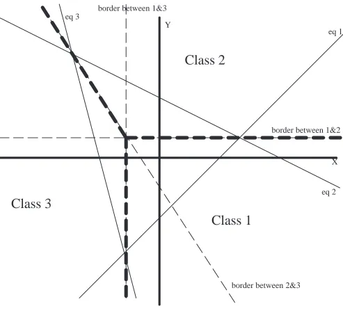
An example LM with the following linear discriminants for 3 classes and how it splits the XY plane is in Figure 8:
LD1 = X – Y – 1 LD2 = X + 2Y – 2 LD3 = –4X – Y – 4
eq 1
eq 2 eq 3
border between 1&2 border between 1&3
border between 2&3
X Y
Class 2
Class 1
Class 3
Figure 8: Linear Machine with Three
Classes
25
polygonal, a further limitation is that each class has one LD function and so it can only deal with a single convex region [14,69].
Without any increase in readability and significant limitations in representational abil-ity, Linear Machines are not a widely used technique.
2.2 Feed–forward Neural Nets
Neural nets (also referred to as “connectionist learning” or “parallel distributed proc-essing” [58]) are designed for implementation on a large parallel systems. The indi-vidual components are small and their algorithms simple, but they each contribute a small piece of the concept and together they accomplish the learning task. Individual-ly, the small pieces of the Neural Network do not “understand” the whole solution or the whole problem, but together they stabilize to a state that classifies the inputs. In practice, the behavior of this distributed system is usually simulated by software. Sarle [59] contends that the most common form of neural networks actually perform simple statistical functions and he gives a brief summary on the relationship between neural networks and statistical regression.
2.2.1 Overview of Feed–forward Neural Nets
Figure 9: Artificial Neuron
The response function of an artificial neuron is usually some sort of function like [39,65]:
or:
(1)
27
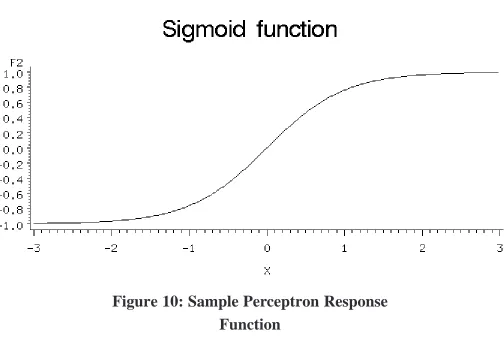
Figure 10: Sample Perceptron Response
Function
These functions both start small with small slope for all small input values and then as the input values approach 0 (or for the perceptron the value approaches the threshold) the slope increases quickly. When the input sum gets very large (with respect to the threshold), the slope again slows down as the function asymptotically approaches the ceiling output of 1.
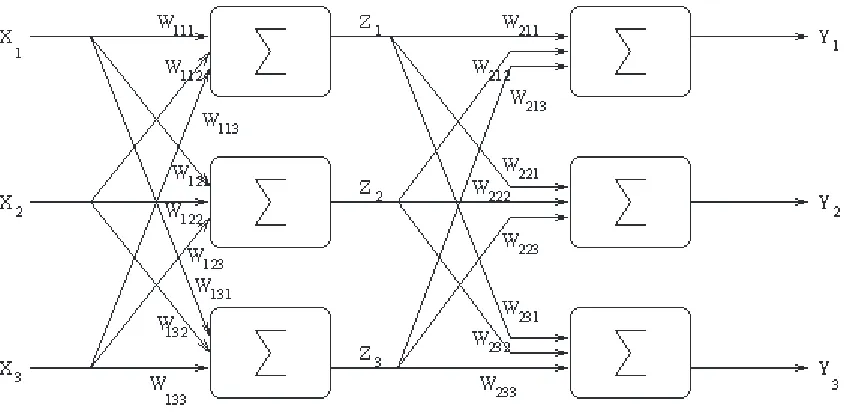
Figure 11: 2–layer neural network
Training the network consists of feeding examples with known responses into the net-work and adjusting the weights on the perceptrons according to the responses that the network gives (rewarding correct responses and discouraging incorrect responses). An error function (with respect to a given set of weights w) is defined as the amount that the network is wrong in its responses. The least squares error is often used [38]:
(2)
where k(X) is the actual class from the training example and y’i is the “guess” from the network. As the network is trained, the thresholds and weights are adjusted according to the accuracy of the network responses until the adjustments become stable and the behavior of the network becomes more constant. The change in the weights is based on the magnitude of the error [38]:
(3)
29
(Eq. 3) moves “downhill” with respect to the error surface, proportionally to the slope of the error gradient. This greedy algorithm is called gradient descent.
This equation works well for a one–layer network where the k’(X) is the encoding of the actual classification for the encoded input X and y is the actual output of the only layer. The g term represents the earlier threshold functions on the sum of the
weighted bits of the encoded input example. This error term is then summed across all of the examples as they are fed into the network.
The sum of the squares is commonly used, but any differentiable function that is 0 when the difference between the output and the real classification is 0 and increases at an increasing rate as the differences increase is sufficient. An alternative is tanh (the hymerbolic tangent) [38] which is a similarly shaped function.
When the error function (Eq. 2) is differentiated, the change to the weights of this unit caused by the kth bit of the ith individual input example becomes [38]:
But this solution is limited to single–layer networks because of the clear effect of the outputs as a function of the weights. However, single layer networks are not sufficient to learn many functions or classes.
The functions that a network can learn are limited by the functions that it can repre-sent, [65], and a single–layer network can learn only a limited set of functions. A function is linearly separable if a single hyper–plane through the A–dimensional space can distinguish the classes. Single layer networks can learn only linearly sepa-rable functions [53].
Two–layer networks can learn any binary function in the inputs and a sufficiently con-nected three–layer network can learn any function on the inputs [53]. But training multi–layer networks is more complicated than training single–layer networks. In a single–layer network, the output of the network is a simple function of the weights and the sigmoid function in the artificial neuron, so the gradient of the error function with respect to the weights is relatively simple. In multi–layer networks, the relationship between the input at the first layer and the output from the last layer be-comes more indirect and the required adjustment to the weights bebe-comes more diffi-cult to calculate as each layer are added.
Back–propagation will be described here for a two–layer network, but the idea can be
extended to more layers.
2.2.2 Back–propagation in Feed–forward Nets
In the case of multi–layer networks, the weights on previous levels cannot be adjusted as a function of the error directly because they do not have direct output to the final output of the network. In back–propagation, the effects of the error surface are worked back through the network to the previous levels so that their weights can be adjusted indirectly as a result of the outputs for the examples [38].
Consider the two–layer model depicted in Figure 11. The input to the first layer is an encoding of the input example X. But these units in the first layer do not produce the output Y, but an intermediate output Z. For a unit in the second layer, it is not the en-coded input example, but the output from the previous layer Z which is input and this second layer produces the output Y.
This means that the updates to the first layer weights cannot simply be a function of the outputs of the network because that layer has no direct connection to the outputs of the network. For hidden layers, where the desired output and the actual inputs are not known this was a problem to differentiate, but back–propagation has made this easier. In this example, the first layer is fed the input vector X and the weighted sum of inputs for this unit is:
and unit j in the first layer outputs:
and the lth unit in the second layer receives those outputs Z from the first layer and calculates a weighted sum of its inputs as:
and the final output from this unit of the second layer is [38]:
31
Substituting this back into Eq. 2, gives us a new error function for the second layer (the output layer):
(4)
where the ws are the weights for the final layer and is still the learning rate (same as Eq. 3). The updates to these weights in the second layer becomes:
where the zs are what was produced by the hidden layer. The values for this are all known and the weights of this second layer can be updated.
Back–propagation then works the error back to the previous layer using the chain rule
of partial derivative.
Since
is just applying gradient descent to the second layer, and
is applying it to
the first layer, the total adjustment to the ws can be calculated as:
all of which are known values once the second layer has been processed.
Working the error back through the network in this manner allows the error function to be differentiable and therefore the error surface can be traversed and multilevel net-works can train and stabilize.
2.2.3 Training Time
The training time of a Neural Net architecture is proportional to the weight space that is being searched. Since the weights can have any values, and the search is in the weight space, this would appear to be an infinite search space. However, there are combinations of weights that will yield the same results, so the size of the search space is really proportional to the number of problems that the network can solve, or the number of functions or concepts that can be represented by the architecture. The volume of the entire weight space is:
where is the probability of a given weight set w and the volume of space that im-plements a given function f is:
where is an indicator function that is true if the weight set implements the func-tion. This framework is described in more detail in [38].
If the function is a typical function in the weight space, then if the percentage of the total weight–space volume that implements the desired function is inversely propor-tional to the number of distinct functions that are in the weight space (or the number of distinct functions that can be implemented by the architecture of the neural net). The Vapnik–Chervonenkis dimension for a class of concepts is a measure of the mag-nitude of that class or family of concepts [53]. For a family of concepts F, the Vapnik–
Chervonenkis dimension DVC(F) is the greatest integer d such that F can distinguish any combination (shatter) of a set of d examples. So the VC–dimension is a measure of the size or complexity order of a family of concepts[37].
For example, if the family of concepts was the set of concepts in the XY plane that can be separated by a single line, then DVC(F) would be 2 because the line could shatter
any set of two points. That is, it could break the two points into any combination. However, a single line could not shatter any set of three points. The points could all be colinear and the single line could not separate any combination
The architecture of a network puts a limit on the family of concepts that it can solve. The concept space that the network must search is proportional to the VC–dimension of the family of concepts that the network can learn. However, this is only an upper bound and the exact relationship is not clear. Hertz, Krogh and Palmer [38] give a de-scription of some of the factors that control how well a network might learn a concept. In practice neural networks can take a long time to train. In an empirical analysis of neural net performance, Weiss and Kapouleas [67] report that 6 months of SUN 4/280 CPU time were used to get the data for their analysis on four different data sets with approximately 6 different configurations for each data set.
33
2.2.4 Concept Limitations
A two–layer neural network can create functions that peak around a desired range in the values of its attributes. By thresholding this peak, the network can create a space of arbitrary size around this peak. By taking combinations of these small regions in the third layer, a shape of arbitrary shape can be formed. So a three–layer neural net can distinguish a region of arbitrary shape to any degree of accuracy [38,53].
A two–layer net can distinguish any binary function on binary inputs [53].
But that isn’t the whole picture. While a three–layer neural net can represent any shape, the idea assumes that there are an infinite number of perceptrons and that they are infinitely interconnected. Since training time is proportional to the VC–dimension and the VC dimension can be exponential, and the VC dimension is dependent on the size of the net, the training time on a fully interconnected network for a large problem may be exponential in the number of inputs.
Also, neural nets in practice sometimes “over train” [18] a concept and do not general-ize outside of the training set [62] Since the concept is not very understandable by hu-mans, it is not easily seen.
It is difficult to analyze how many perceptrons are required for a given level of accu-racy [38,41]. The construction method described above only shows that a neural net
could learn a concept. It is not necessarily the way the network would solve it. For
example, suppose we were trying to learn the concept “x<y” in Cartesian space. The method described in [53] would require a lot of perceptrons to create round shapes along the axis, but a single perceptron can learn that concept with a simple linear com-bination of x and y (y–x and a threshold of 0).
For arbitrary shapes, it is difficult to determine a priori what state the weights will sta-bilize to or how complicated the network will have to be to achieve a specified level of accuracy. If the VC–dimension of the family of concepts was known, then the com-plexity of the required network might be estimated. But for a given problem and/or architecture, it is difficult to predict the training time or accuracy ahead of time.
2.3 AI Methods Not Addressed
2.3.1 Bayesian Nets
A Bayesian net is an annotated directed acyclic graph [34] in which each node repre-sents a probability distribution of a set of mutually exclusive and exhaustive states from some subset of the attributes. (The attributes in a Bayesian net may be derived attributes rather than directly measured attributes.) The information about these states or values then lead into other nodes. Knowledge about these attributes cause mes-sages to be sent through arcs to create more refined probability distributions of states that are influenced by these values. The structure of the net encodes priority and pre-cedence information on the values of some of the attributes.
The advantages of Bayesian nets over decision trees (and their derivatives) are that: 1 They deal well with missing information. Since each edge describing values of the attributes leads to a fully complete probability distribution, missing data is simply not used in the calculation.
2 They give a probability vector for the dependent attribute (or class), so they give a confidence level to the classification [32,46].
3 The structure of the net can encode precedence information about the mutual ex-clusivity of certain attribute values and take it into account in the probability dis-tribution.
4 The probability distribution of the states also contains probabilities of the attribute variables, so the structure is more flexible with respect to the target variable. As more work is being done in fuzzy logic and reasoning under uncertainty, Bayesian nets are the basis for many new techniques [7,46].
However, these advantages are outside the scope of this examination since they do not fit the paradigm described in Section 1.2. Also, the representational limitations of the
concept itself are the same as for decision trees. While the probability density
func-tions at the nodes could be continuous funcfunc-tions, they are usually stored as conceptual tables of the attribute alternatives. Continuous attributes are thresholded and turned into classification alternatives. This has the same effect of breaking the space down with orthogonal hyperplanes similarly to decision trees.
2.3.2 Regression Trees
35
To estimate the value for a new example, the decision tree is followed except that the leaf node is a regression formula.
2.3.3 Inductive Logic Programming (ILP)
Inductive Logic Programming (ILP) uses predicate calculus to represent known con-cepts applies rules to these concon-cepts to derive new concon-cepts. In ILP (or predicate cal-culus), a concept c can be formalized as a subset of the objects in the universe of discourse U [47]. Unlike most inductive techniques, ILP allows relational expressions between concepts. In ILP the problem statement contains:
a set P of possible programs (the program space P combined with the background knowledge makes up the hypothesis space H) a set X+ of positive examples
a set X– of negative examples
a consistent logic program b, such that: b x+, for at least 1 x+ ∈ X+ and the ILP method will try to find:
a logic program h ∈ H, such that b ∪ h is complete and consistent. So P is the program space that is being searched. X+ is a set of examples that are known to be true for some concept and X– is a set of examples that are known to be false for this concept. b (often referred to as background knowledge) is a set of ground clauses or relationships that are known to be true but are not sufficient to ex-plain all of the positive examples.
Unlike the other machine learning methods discussed, ILP usually uses Prolog or First Order Predicate Calculus (FOPC) as its representational base. This allows relational concepts to be expressed that would be difficult to exhaustively represent with a finite set of examples. For background on FOPC, see [17].
ILP uses bottom–up methods of generalization and top–down methods of specializa-tion to create new clauses or concept representaspecializa-tions.
Bottom–up methods take pairs of specific concepts and try to create the most specific clause that entails the original two clauses. It then repeats this generalization process with more and more positive examples until it has a concept generalization that in-cludes all of the positive examples but is as specific as it can be.
as not to entail the negative examples. When it has made the clause specific enough to not include any negative examples, the remaining clause is the learned concept.
Since ILP uses predicate logic, it can represent richer concepts, but it does not deal well with numeric data and is not easily compared to decision trees or neural nets. Decision trees, neural nets, ILP and Bayesian nets are the major AI techniques used in common practice [48].
2.4 Summary of AI Methods
In general, an AI technique differs from a statistical technique because it tries to create a legacy description of the concept. This has an advantage in running future examples through the legacy rather than having to go through the entire data set for each new example. It is also useful in trying to glean additional information about the concept being learned. The concept description can help the user gain insight into the nature of the concept.
However, the representational limitations of the learning method and the process by which the concept is learned will usually add a degree of inaccuracy to the concept. Hybrid systems that combine more than one AI technique try to overcome the limita-tions of some of the individual techniques. Baldwin, Martin and Pilsworth [6] use Ko-honen nets [44] to create classification clusters so that numeric attributes can be
represented nominally. Peng and Zhou [54] mix neural computing with uncertainty. In general, classification trees and neural nets are the most common methods. Deci-sion trees are the simplest and easiest to understand, but they are not as accurate as neural nets and they do not deal with missing data as well as Bayesian nets.
37
Chapter
3.
Statistical Methods of
Classification
This chapter will describe some statistical methods for classification. In general, sta-tistical methods differ from AI methods in that they make no attempt to generate a representation of the concept.
The most common statistical methods fall into two categories. Methods in the first category create a direct statistical model to predict a binary outcome variable. These methods include logistic regression and the probit model [40]. Methods in the second category try to determine the most likely class of an example by estimating the proba-bility density function of all of the classes. Methods for estimating distributions in-clude parametric methods, non–parametric kernel methods, nearest neighbor methods and regression splines [30]. With the nearest neighbor methods, the example is classi-fied by voting among either the n nearest neighbor points or by voting among all points within a specified radius. These are both simple cases of the non–parametric kernel methods and won’t be discussed in detail here.
Splines are used to estimate a distribution, but are usually applied to a single dimen-sion and are not normally applied to classification.
3.1 Direct Model Methods of Statistical
Classification
3.1.1 Logistic Regression
In logistic regression, the response variable is a binary outcome variable (like a classi-fication) and the independent variables are the attributes of the example space [40]. Unlike a normal linear regression, the response variable cannot be a linear combina-tion of the independent variables because it has only two outcomes. The output of the logistic regression formula is the predicted probability that the actual outcome is 1. This output (like any probability) is still restricted to be between 0 and 1.
Normal linear regression and logistic regression are both part of a family of general linear models (GLMs). In general linear models, the dependent variable Y is esti-mated by some function of a linear combination of the dependent variables [40]:
where:
The s are coefficients and the Xs are the values of the attributes. With logistic re-gression, the function G is something like:
which is always between 0 and 1 and is monotonic in the parameter . The function
is also symetric in that G(X) = 1–G(–X) so that predicting positive examples will
39
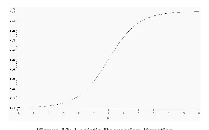
Figure 12: Logistic Regression Function
The calculation is to find the optimal vector to minimize the error of the function. This is done by maximizing the probability that the estimate will be correct. In order to do this, the likelihood function must be constructed. This function is equal to the probability of the observed values given the data. The s for which this function is maximized are the s with the least probability of errors.
If Y is the binary outcome for a given example and is the estimated probability of Y being 1, and the quantity is the estimated probability that Y is 0. The likeli-hood function is then:
for each X attribute. The total likelihood function for a multivariate system is:
Since the function is maximized whenever the log is maximized, the log of the func-tion is taken as:
When the function is differentiated, and set to 0, the resulting likelihood equations are:
and
These equations are solved using an iterative method [40].
The method is parametric in the sense that the formula is known and the calculation is to determine the parameters (the s). The assumption that this parametric form im-plies is that the probability of the outcome is monotonic in any of the attributes and there are no interactions between the terms. These assumptions are common to any GLM [1]. As with normal linear regression, the user may add quadratic and higher order terms to overcome parts of these limitations, but the user must be aware of these relationships in order to add these terms. The method will not find these relationships on its own.
3.1.2 The Probit Model for Binary Outcomes
The probit model is based on the idea of a tolerance distribution of the subjects on the attribute. Each example has a different tolerance for the attribute in question before the attribute will cause a change in classification of the example. Let x be the dosage of a toxic chemical and T be the threshold of the subject. The response (bad effect) will be 1 if and only if x>T. Since T is assumed to be approximately normal, then the probability that x>T is equal to the CDF (Cumulative Density Function) of a normal distribution of the tolerances with the appropriate mean and variance [1].
Mathematically this works out as a sigmoid shaped function similar to the logistic re-gression function, but the basis of it is different. The basis is also somewhat different than most of the AI paradigms in that it does not divide space to get the mapping, but assumes a variation in the tolerance of the subjects or examples.
For a single attribute x predicting the probability of the binary outcome y is:
41
also makes the assumption that the probability of the outcome is monotonic in the at-tribute values.
3.2 Classification by PDF Estimation
When classifying by PDF estimation, the classification problem is turned into a more general problem of estimating the underlying distribution of a set of sample points. Since the sample is a set of discrete points assumed to have come from some continu-ous function, the problem is to estimate what the underlying continucontinu-ous probability density function (PDF) is. Since the underlying distribution has randomness to it, there is some probability that the points can come from any distribution with the same range. The problem is to find the distribution that is most likely to have produced the examples [35].
Estimating the PDF can then be used for classification. Given the underlying PDF and frequency for each class, the new point can be classified as the class that is most likely at that point in the attribute space.
In parametric discriminant functions, certain characteristics of the underlying dis-tribution are assumed to be known (Usually it is presumed to be multivariate normal, but it can be assumed to be from any family of distributions.) and the points for a giv-en classification are assumed to be from this distribution. The specifics of the dis-tribution (such as mean and variance for the multivariate normal) are then calculated. For classification, this is done for each of the classifications. A new point is classified based on its class–specific probabilities from the estimated PDFs.
Non–parametric methods try to recreate the function from which the points are drawn
without assuming anything about the underlying distribution. There is no attempt to fit the example points into a formula or estimate the formula for the entire PDF. The estimate is made from the combined weight of the sample points. The idea that these underlying distributions can be arbitrarily complex is common in AI.
3.2.1 Parametric Methods of PDF Estimation
that once the parameters of the function are estimated, they represent a sort of con-cept, and the underlying data can be discarded [35].
If the family of distributions is known (the general type), then there exists some set of parameters that describe the distribution in detail. For multivariate normal, this would be the multivariate mean vector and the variance–covariance matrix . An estimator is a method or formula to calculate the unknown parameter . If a para-meterized model is used, then the model has the following properties:
Bias. The bias of an estimator of parameter is:
If the expected value of the parameters, E(’) = then is unbiased.
Consistency. An estimator ’ of a parameter is said to be consistent if ’ converges in probability to .
where n is the sample size on which is based.
Efficiency. An estimator ’ of a parameter is said to be efficient if for a given sam-ple size it has the smallest variance of all estimators of .
Sufficiency. An estimator ’ of a parameter is said to be sufficient if the estimator can be used in place of with some level of accuracy. For a further definition, see Hand [35].
Robustness. An estimator is robust if it is still reasonably accurate even if the
para-metric assumptions are not completely accurate.
In a parametric estimation there could be any unknown parameter. The parametric method might assume a threshold, or that the concept is a circle and the parameters are the center and radius of the circle. However, it is usually the distribution family that is known and the parameters that are being estimated are the parameters of the dis-tribution, like mean and variance.
Once the parameterized distributions have been estimated, the PDF for class i at vec-tor x ( ) can be calculated. Bayes theorem implies that:
where p(x) is the global PDF at vector x. The predicted class is just the class with the highest probability.
43
truly of the form that is being estimated, then the distributions with the parameters should give accurate estimations of the PDFs at any point.
The problem with parameterized methods is that for many data sets, either the general form of the PDF is unknown, or the underlying distribution does not have a simple form that lends itself to the parameterized method.
As long as the underlying distributions fit the assumptions made by the model, these parametric estimators work well, but they are very sensitive to violations of the as-sumptions.
A common assumption for the parametric estimator is that the underlying distribution is a multivariate normal distribution. The mean vector and covariances matrix are cal-culated and there is a simple approximation for the PDFs. For any other family of dis-tributions, the appropriate parameters must be calculated. Along with the frequencies, there is a simple way of estimating (for any point in the attribute space) which class is most likely.
For example, suppose the domain of the problem is the unit square on the XY plane and there are three classes of interest. The three classes have equal frequencies and the mean vectors and covariance matrices from the training set are calculated as:
Figure 13: Parametric Class
Map-ping – Good Example
This mapping assumes that the frequencies of examples in the different classes are equal. When classifying using this method, the relative frequencies are taken into ac-count to yield a raw probability value that the new example fits into each class. The class with the highest raw probability is the ’guess’ of the estimator.
If the actual underlying distributions are normal or nearly normal, then this method works well. Figure 13 shows a reasonable and clear mapping of the three regions. But if the assumptions are not met, then this method may have poor results.
45
(.573,.073) to (.927,.427), from (.073,.573) to (.427,.927) and from (.573,.573) to (