Uncertainty-based learning of acoustic models from noisy data

(1)

Uncertainty-based learning of acoustic models from

noisy data

Alexey Ozerov, Mathieu Lagrange, Emmanuel Vincent

To cite this version:

Alexey Ozerov, Mathieu Lagrange, Emmanuel Vincent. Uncertainty-based learning of acoustic

models from noisy data. Computer Speech and Language, Elsevier, 2013, 27 (3), pp.874-894.

<10.1016/j.csl.2012.07.002>.

<hal-00717992v2>

HAL Id: hal-00717992

https://hal.inria.fr/hal-00717992v2

Submitted on 17 Apr 2013

HAL

is a multi-disciplinary open access

archive for the deposit and dissemination of

sci-entific research documents, whether they are

pub-lished or not.

The documents may come from

teaching and research institutions in France or

L’archive ouverte pluridisciplinaire

HAL

, est

destin´

ee au d´

epˆ

ot et `

a la diffusion de documents

scientifiques de niveau recherche, publi´

es ou non,

´

emanant des ´

etablissements d’enseignement et de

recherche fran¸

cais ou ´

etrangers, des laboratoires

(2)

Uncertainty-based Learning of Acoustic Models from

Noisy Data

1

Alexey Ozerov 1_{, Mathieu Lagrange}2_{, and Emmanuel Vincent}3

1

Technicolor Research & Innovation, France

2

STMS - IRCAM - CNRS - UPMC

3

INRIA, Centre de Rennes - Bretagne Atlantique

[email protected], [email protected], [email protected]

Abstract

We consider the problem of acoustic modeling of noisy speech data, where the uncertainty over the data is given by a Gaussian distribution. While this un-certainty has been exploited at the decoding stage viauncertainty decoding, its usage at the training stage remains limited to static model adaptation. We in-troduce a new Expectation Maximisation (EM) based technique, which we call

uncertainty training, that allows us to train Gaussian mixture models (GMMs) or hidden Markov models (HMMs) directly from noisy data with dynamic un-certainty. We evaluate the potential of this technique for a GMM-based speaker recognition task on speech data corrupted by real-world domestic background noise, using a state-of-the-art signal enhancement technique and various uncer-tainty estimation techniques as a front-end. Compared to conventional training, the proposed training algorithm results in 1% to 2% absolute improvement in speaker recognition accuracy by training from either matched, unmatched or multi-condition noisy data. This algorithm is also applicable with minor modi-fications to maximum a posteriori (MAP) or maximum likelihood linear regres-sion (MLLR) acoustic model adaptation from noisy data and to other data than audio.

Keywords: Noisy data, training, uncertainty, classification, acoustic model, Gaussian mixture model, hidden Markov model, expectation-maximization

1. Introduction

Classification and detection systems often face a variety of distortions (e.g., additive or convolutive) resulting in noisy data. In order to achieve noise robust-ness, at least three complementary approaches can be taken. At the signal level, one can apply enhancement techniques such as noise suppression (Ephraim,

1

This work was performed while A. Ozerov was with INRIA and partly supported by OSEO, the French State agency for innovation, under the Quaero program.

(3)

1992), source separation (Vincent et al., 2012) or dereverberation (Delcroix et al., 2009). At the feature level, one can define features that are robust to the considered type of noise or to the residual noise after enhancement (Nadeu et al., 1997). Finally, at the classifier (or decoder) level, one can account for possible distortion of the features within the classifier itself. In this paper, we focus on the latter approach by considering the problem of acoustic modeling of noisy speech data using Gaussian mixture models (GMMs) or hidden Markov models (HMMs).

The most straightforward approach to increasing the accuracy of the classi-fier is to train the models overmatched training data exhibiting the same type and amount of noise as the test data (Droppo and Acero, 2008). Unfortunately, such data are not always available and one may be constrained to use clean,

multi-conditionor evenunmatched training data whose noise characteristics do not match those of the test data. This is an example of the general problem

known asconcept shift in the machine learning community whereby the noise

contribution varies between the training and test datasets (Moreno-Torres et al., 2012). One approach to this problem consists of clustering the model compo-nents and adapting their means and covariances within each cluster via a static (time-invariant) transform (Deng et al., 2000; Gales, 2011). This approach ac-counts for theuncertaintyover the data induced by noise, but it does not exploit estimates of this uncertainty that may be available from the signal enhancement front-end and it is restricted to rather stationary noise environments by design. More recently, several approaches have been proposed to dynamically adapt the model parameters in each time frame in response to nonstationary noise. A separate signal enhancement front-end is employed that allows the use of har-monicity cues and spatial cues, which are essential for signal enhancement but not modeled by feature-domain GMMs or HMMs. The uncertainty over the data is then typically encoded either by a set of binary flags indicating whether each data dimension is “observed” or “missing” (Cooke, 2001) or by a Gaussian distribution whose mean and covariance matrix represent, respectively, the es-timated underlying clean data and noise covariance (Deng et al., 2005). This last approach is the most flexible, since it allows to the amount of noise to be quantified along with the noise correlation between different data dimensions in each time frame. In the following, we focus on this approach, which has been successfully employed by the best scoring system (Delcroix et al., 2011) of the 2011 CHiME Speech Separation and Recognition Challenge (Barker et al., 2013).

While several algorithms have been derived that exploit uncertainty over the test data (Cooke, 2001; Barker et al., 2005; Deng et al., 2005; Srinivasan and Wang, 2007; Delcroix et al., 2009; Shao et al., 2010; Kolossa et al., 2010), uncertainty over the training data has not been fully exploited so far. Most approaches (Cooke, 2001; Barker et al., 2005; Deng et al., 2005; Srinivasan

and Wang, 2007; Shao et al., 2010) assume conventional training from clean

data. This training strategy is not always applicable in the case of, e.g., field recording or mobile recording where the whole recording might be corrupted by noise. Also, even when sufficient clean data are available for training, the

(4)

uncertainty over the test data is never perfectly estimated in practice such that some noise may remain that is not accounted for. Recently, Delcroix et al. (2011) and Kolossa et al. (2011) achieved better results byconventional training from noisy data. Nevertheless, this heuristic strategy remains sensitive to mismatched training and test noise conditions and, even in matched conditions, the noise variance is overestimated by a factor of two. Indeed, the noise is taken into account both at the training stage within the model parameters and at the decoding stage within the uncertainty and these two contributions add up. Liao and Gales (2007) proposed a more principled training algorithm for use with static model adaptation, but the exploitation of dynamic Gaussian uncertainty over the training data remains an open issue.

In order to address this issue, we introduce a new EM based technique that allows us to train GMMs and HMMs directly from noisy data with dynamic Gaussian uncertainty. By analogy with theuncertainty decoding algorithm of Deng et al. (2005), we refer to this training strategy asuncertainty training. The proposed algorithm generalizes both the algorithm of Ghahramani and Jordan (1994) for binary uncertainty and the algorithm of Arberet et al. (2012) for Gaussian uncertainty with diagonal covariance and zero-mean GMMs with di-agonal covariances, which were applied in different contexts. Furthermore, it is also applicable with minor modifications to maximum a posteriori (MAP) (Gau-vain and Lee, 1994) or maximum likelihood linear regression (MLLR) (Leggetter and Woodland, 1995) model adaptation and to other noise-corrupted data, e.g., microarray data for which different genes and different conditions have differ-ent levels of experimdiffer-ental and biological noise whose variance can be estimated (Sanguinetti et al., 2005). This article expands our preliminary paper (Ozerov et al., 2011) by providing more insight about the proposed GMM training algo-rithm, by extending it to HMMs, and by extensively evaluating it for a speaker recognition task with real-world data and uncertainty estimates as opposed to synthetic data and oracle (i.e., ideal) uncertainty. For the sake of conciseness, we focus on GMMs in most of the paper and in the experimental study, and we present the algorithm for HMMs in Appendix B.

As a by-product, we also introduce the following two new uncertainty esti-mators. For the particular task and signal enhancement algorithm employed, we show that one of the best uncertainty estimators among the variety of estimators considered here is obtained by computing the uncertainty resulting from multi-channel Wiener filtering (Fischer and Kammeyer, 1997) in the time-frequency domain and propagating it to the Mel Frequency Ceptral Coefficient (MFCC) domain using Vector Taylor Series (VTS) (Moreno et al., 1996). Moreover, for benchmarking purposes, we introduce an oraclerank-1 uncertainty covariance estimator that outperforms the classical oracle diagonal covariance estimator.

The rest of the paper is organized as follows. In Section 2, we introduce the notations and briefly recall the state-of-the-art GMM-based generative clas-sification approach including uncertainty decoding. The proposed uncertainty training EM algorithm is then described in Section 3. An exhaustive evalua-tion of this algorithm is conducted in Secevalua-tion 4 for a speaker recognievalua-tion task. Finally, we draw some conclusions in Section 5.

(5)

2. GMM-based classification and uncertainty decoding 2.1. Conventional training and decoding

Classification is the problem of assigning a sequence ofM-dimensional real-valued vectorsy={yn}Nn=1 to a classC. In the context of audio, the observed vectors are typically feature vectors, e.g., MFCCs, each describing one frame of

audio. Each classC is modeled by one GMM as

p(yn|θ) = XI

i=1ωiN(yn|µi,Σi), (1) wherei= 1, . . . , I are Gaussian component indices, µ_i, Σi and ωi (P_iωi = 1)

are respectively the mean, the covariance matrix and the weight of the i-th component,θ,{µ_i,Σi, ωi}Ii=1 denotes the set of GMM parameters2, and

N(yn|µi,Σi), 1 p (2π)M_|_Σ i| −(yn−µi) T_Σ−1 i (yn−µi) 2 . (2) Under this model, the likelihood of the observed sequenceyis given by

p(y|θ) =YN

n=1p(yn|θ), (3) and, introducing latent componentsqn (n = 1, . . . , N), the model can be also

written as

(yn|qn =i)∼ N(µi,Σi), P(qn=i) =ωi. (4)

Using this formulation, conventional GMM-based generative classification consists of the following two steps (Reynolds, 1995):

1. Training (or adaptation): For each classC the corresponding model pa-rametersθ are estimated from some sequence of training vectors by max-imizing the likelihood (3). This step may be replaced or completed by an adaptation step from some adaptation data, where the maximum likeli-hood (ML) criterion (3) is replaced by MAP or MLLR.

2. Decoding: For each test sequence y, the likelihood (3) is computed for all classesC and, assuming a uniform class prior (p(C)∝1), the class is selected for which it is maximum.

Training is typically performed via the EM algorithm (Dempster et al., 1977), considering the Gaussian component indices q={qn}Nn=1 as latent data. The resulting EM updates are summarized in Algorithm 1.

2.2. Gaussian uncertainty decoding

In the case of noisy data, it is assumed (Deng et al., 2005; Delcroix et al., 2009; Kolossa et al., 2010) that the observed noisy data, denoted as ¯yn, are

2

(6)

Algorithm 1One iteration of the conventional EM algorithm (Dempster et al., 1977) for GMM training from clean or noisy data.

E step. Compute conditional expectations of natural statistics:

γi,n∝ωiN(yn|µi,Σi), and X

iγi,n= 1. (5)

M step. Update GMM parameters:

ωi = 1 N N X n=1 γi,n, (6) µi= 1 PN n=1γi,n N X n=1 γi,nyi,n, (7) Σi= 1 PN n=1γi,n N X n=1

γi,nyi,nyTi,n−µiµTi , (8)

and, in caseΣi is constrained to be diagonal, set its off-diagonal elements to

zero.

distributed as

(¯yn|yn)∼ N(yn,Σ¯y,n), (9)

where yn are the underlying clean data, which are themselves distributed

ac-cording to a GMM, and ¯Σy,nis the noise covariance matrix3. The corresponding

Bayesian network representation is shown in Fig. 1. Here and in the following, noise may refer either to the original acoustical noise corrupting the features or to the residual noise after signal enhancement as depicted in Fig. 2. A num-ber of techniques have been proposed to estimate diagonal or full uncertainty covariance matrices from single-channel or multi-channel data either directly in the feature domain (Delcroix et al., 2009) or by propagation of time-frequency domain uncertainty estimates (Kolossa et al., 2010).

Since the clean datay are not exactly known, one cannot directly compute the likelihood (3). It is hence modified by marginalizing over the clean data as

3

Note that this model assumes zero-mean noise. This assumption does not reduce the generality of the approach since, in the case of a noise with nonzero mean ¯µe_,n, one may

simply consider ¯yn−µ¯e,n instead of ¯yn. In the case of uncertainty propagation from the

STFT domain to the feature domain (see Section 4.1.4), ¯yndepends on the chosen uncertainty

propagation technique and generally differs from the features computed without uncertainty propagation.

(7)

GMM Hidden clean _feature _featureNoisy

Figure 1: Bayesian network representing the distribution of noisy features with Gaussian uncertainty.

Figure 2: Block diagram of Gaussian uncertainty decoding.

(Deng et al., 2005; Kolossa et al., 2010):

p(¯y|Σ¯y, θ) = Z RM×N p(¯y|y,Σ¯y)p(y|θ)dy (10) = N Y n=1 I X i=1 ωiN(¯yn|µi,Σi+ ¯Σy,n), (11) where ¯y={y¯n}Nn=1, ¯Σy= _¯ Σy,n N

n=1, and (11) is derived from (10) using the fact that the density function of the sum of two independent random vectors (hereen,y¯n−yn andyn) is the convolution of the density functions of these

vectors (Grinstead and Snell, 1997). Since the variance of independent events adds up, the effect of the noise is to widen the mixture components by ¯Σy,n. The

likelihood (11) can readily be used at the decoding stage, resulting in so-called uncertainty decoding.

3. Proposed uncertainty training algorithm

As discussed in the introduction, state-of-the-art approaches typically train the models either from clean data, as shown in Fig. 3A, or from noisy data, as shown in Fig. 3B, using the conventional training strategy in Section 2.1. By contrast, as shown in Fig. 3C, we propose to train the models over noisy data by maximizing the modified likelihood (11) that accounts for data uncertainty.

(8)

Figure 3: Block diagrams of the state-of-the-art and proposed training strategies.

Contrary to the conventional likelihood (3), the modified likelihood (11) does not explicitly describe the clean datay. Thus, in order to derive an EM algorithm maximizing this likelihood, the latent data including the component indices q are taken together with the clean data y: B , {y,q}. Denoting by A , {y¯} the observed data, it can be shown that the distribution of the

complete data{p(¯y,y,q|θ)}θ (which is a product of Gaussian and discrete

dis-tributions) belongs to theexponential family (Dempster et al., 1977) and that the sett(y,q) =t0

i,n,t1i,n,T2i,n _i,n defined by

t0_i,n,δ(qn, i), t1i,n,δ(qn, i)yn, T2i,n,δ(qn, i)ynyTn, (12)

where δ(i, j) is the Kronecker delta function, is a set of natural (sufficient) statistics (Ozerov et al., 2007) for this family.

One iteration of EM then consists of

• E step: computing the expectation of the natural statistics conditionally on the current parameter estimates , and

• M step: re-estimating the parameters from the updated natural statis-tics by maximizing the conditional expectation of the complete data log-likelihoodQ(θ|θ′) =RB[logp(A,B|θ)]p(B|A, θ

′

)dB.

The resulting updates are given in Algorithm 2. For detailed derivation, please refer to Appendix A. Note that the uncertainty covariances ¯Σy,n and the

(9)

Algorithm 2One iteration of the proposed uncertainty training EM algorithm for GMM training from noisy data.

γi,n∝ωiN(¯yn|µ_i,Σi+ ¯Σy,n), and X iγi,n= 1, (13) ˆ yi,n=Wi,n(¯yn−µi) +µi, (14) b

Ryy,i,n= ˆyi,nyˆTi,n+ (I−Wi,n)Σi, (15)

where Wi,n=Σi Σi+ ¯Σy,n −1 . (16)

M step. Update GMM parameters:

ωi = 1 N N X n=1 γi,n, (17) µ_i=_PN1 n=1γi,n N X n=1 γi,nˆyi,n, (18) Σi= 1 PN n=1γi,n N X n=1 γi,nRbyy,i,n−µiµTi, (19)

and, in caseΣi is constrained to be diagonal, set its off-diagonal elements to

zero.

no constraint that they share the same structure. An analogous algorithm for uncertainty training of HMMs is summarized in Appendix B.

In Algorithm 2, the uncertainty covariances ¯Σy,n are exploited not only to

compute the posterior component probabilitiesγi,nin (13) as with uncertainty

decoding, but also to compute the expectations ˆyi,n and Rbyy,i,n in (14) and

(15) in the E step. These expectations are actually the first and second order moments of the underlying clean data, which are estimated by the Wiener filter

Wi,n in (16). This filter is characterized by the covarianceΣiof the clean data,

as modeled by the GMM, and the covariance ¯Σy,n of the noise, as modeled by

the uncertainty. Given these moments, the M step is essentially the same as in Algorithm 1.

In other words, the proposed algorithm alternately estimates the underlying clean data and their distribution. Contrary to conventional training on noisy data, the estimated model parameters are therefore theoretically noise-free. In practice, they may still be affected by noise to a smaller extent, due to inaccurate estimation or modeling of the input uncertainty.

It can easily be shown that the updates in Algorithm 2 are “asymptoti-cally” identical to those of the EM algorithm for binary uncertainty proposed in (Ghahramani and Jordan, 1994) in the case when the uncertainty covariances

(10)

¯

Σy,n are diagonal with either zero entries for observed data or +∞entries for

missing data, as well as to the conventional EM updates in Algorithm 1 in the case when all uncertainty covariances ¯Σy,n are zero. Moreover, although the

proposed algorithm is presented in the context of GMM or HMM training, it can easily be modified to perform MAP/MLLR adaptation, since only the M step should be modified as in (Gauvain and Lee, 1994; Leggetter and Woodland, 1995), while the E step remains unchanged.

The computational cost of the proposed approach is comparable to that of conventional training in the case of diagonal uncertainty covariances. In the case of full uncertainty covariances, the cost of each iteration significantly increases

due to the inversion of an M ×M full matrix for each time frame and each

Gaussian component, but it remains similar to that of uncertainty decoding in this case.

4. Evaluation

We evaluate the proposed uncertainty training algorithm for a speaker recog-nition task on speech data corrupted by real-world domestic background noise, using a state-of-the-art signal enhancement technique and various uncertainty estimation techniques as a front-end. We mostly follow the methodology de-scribed in the well recognized work of Reynolds (1995) for clean data. We acknowledge that it does not constitute the state-of-the-art method for tackling speaker recognition today. However it provides a simple proof of concept and enables us to focus on the choice of the training, test and uncertainty estimation algorithms as opposed to the settings of the signal enhancer and the classifier. The data and the software used for this experiment are released in our open

sourceAcoustic Model Uncertainty Learning Experimental Toolbox (AMULET)

(Ozerov et al., 2012a) together with a user guide and examples of use.

4.1. Test methodology

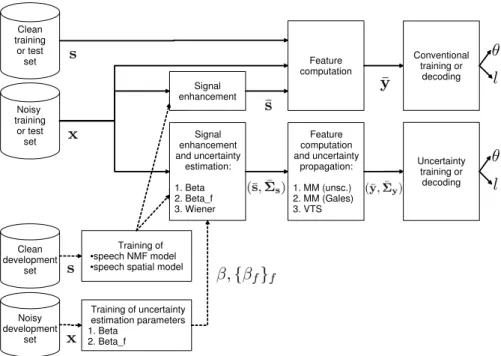
To simplify understanding of the various steps detailed below, the overall test methodology is depicted in Figure 4.

4.1.1. Data

We built a training set, a development set, and a test set by adding binaural reverberated clean speech and background noise from the CHiME training cor-pus (Barker et al., 2013)4_{. Each of the three datasets involves 680 utterances} of approximately 1.5 second duration spoken by 34 speakers (20 sentences per speaker) and continuous domestic background recordings including, e.g., inter-fering speakers, TV, outside traffic noise or footsteps. All signals are sampled

4

Since clean speech, which is needed later on for benchmarking, was unavailable for the test dataset, we built our own datasets from the original CHIME training dataset such that they have almost the same characteristics as the CHiME test and development datasets.

(11)

Signal enhancement and uncertainty estimation: 1. Beta 2. Beta_f 3. Wiener Noisy training or test

set _computationFeature

and uncertainty propagation: 1. MM (unsc.) 2. MM (Gales) 3. VTS Signal enhancement Feature computation Conventional training or decoding Uncertainty training or decoding Noisy development set Clean training or test set Clean development set Training of •speech NMF model •speech spatial model

Training of uncertainty estimation parameters 1. Beta

2. Beta_f

Figure 4: Block diagram representation of the test methodology. Datasets and processing blocks are represented as cylinders and rectangles, respectively. One training or test setup corresponds to a single (left to right) pass through the solid arrows and to a choice of one method from each enumerated list. Certain parameters of the signal enhancement and the uncertainty estimation techniques are pre-trained from development datasets as depicted by the dashed arrows.

at 16 kHz. The utterances and the background recordings were randomly se-lected in such a way that no utterance can be found in two datasets and that the background recordings in different datasets were recorded on different days. As such, the background noises in different datasets feature similar acoustical events but the actual signals are distinct.

For each clean speech utterance, different background excerpts of the same length as the utterance were selected according to seven signal to noise ratios (SNRs)5_{: -6, -3, 0, 3, 6, and 9 dB and +}_∞ _{(clean). The clean speech signal} was then added to the selected background signals, resulting in 7×680 = 4760 mixtures per dataset. In line with the CHiME challenge (Barker et al., 2013), we kept track of the temporal position of the selected background excerpts within the continuous background, which enabled us to exploit the surrounding background signal for signal enhancement as in (Ozerov and Vincent, 2011).

5

Note that, in line with the original CHiME data, no signal scaling was performed to achieve a desired SNR. Instead, for every utterance, we randomly browsed the background noise until we found a time interval leading to an SNR within±_{1 dB of the desired SNR.}

(12)

4.1.2. Signal enhancement

Signal enhancement is performed via the state-of-the-art algorithm of Ozerov and Vincent (2011), as implemented using the Flexible Audio Source Separation

Toolbox (FASST)6 _{(Ozerov et al., 2012b). This toolbox allows the user to}

specify the desired spectral and spatial signal models for each sound source from a library of models. Contrary to the use of speaker-dependent models in (Ozerov and Vincent, 2011), target speech is modeled here by a 256-component speaker-independent nonnegative matrix factorization (NMF) spectral model. Background noise is modeled as the sum of 4 sources, each of which follows an 8-component NMF spectral model. In addition, all sources are assumed to follow a rank-1 spatial model. The NMF spectral patterns and the parameters of the spatial model are first trained either on clean speech from the development set or on 20 s of surrounding background noise from the test set (10 s before and 10 s after each utterance)7_{. The former are then kept fixed, while the latter} are adapted to the test mixture in an unsupervised fashion. The NMF temporal activations are randomly initialized and inferred from the test mixture. Finally, the binaural target speech signal is extracted by multichannel Wiener filtering. The effectiveness of this signal enhancement algorithm is evaluated in Appendix E.1 using standard source separation metrics.

4.1.3. Feature computation

After enhancement, both the binaural mixture signals and the enhanced binaural target speech signals are downmixed to mono by adding both channels together and converted into the time-frequency domain using the STFT with a window size of 1024 samples and 512 samples overlap. 19 MFCCs (2nd to 20th coefficients) are computed for each time frame using the Auditory Toolbox (Slaney, 1998) with default settings. The first MFCC was excluded since it is strongly affected by noise and contains little information about speaker identity.

4.1.4. Uncertainty estimation

The uncertainty over the MFCC features is then estimated using a number of state-of-the-art or novel estimators that we present here. Uncertainty estimation techniques typically consist of the following two steps shown in Fig. 2:

1. estimate uncertainty ( ¯Σs) in the complex-valued STFT domain, and

2. propagate it through the corresponding (usually non-linear) feature trans-form.

STFT-domain uncertainty estimation. In the STFT domain, Kolossa et al.

(2010) define the uncertainty covariance as a diagonal matrix ¯Σs,n =

6

http://bass-db.gforge.inria.fr/fasst/

7

Training from surrounding background is in fact an adaptation process that is feasible to apply during test recognition (Barker et al., 2013).

(13)

0 1 2 3 4 5 6 7 8 10−3 10−2 10−1 100 101 Frequency (kHz) Beta_f Beta = 0.073

Figure 5: Scaling factors for the STFT-domain uncertainty estimation technique of Kolossa et al. (2010) and the proposed frequency-dependent variant, as optimized on the development set.

diagn[¯σs2,f n]f o

whose entries are given by ¯

σs2,f n(β) =β|s¯f n−xf n|2, (20)

where the scaling factorβ is optimized on ground truth data as

β= arg min β′ X f,n(¯σs,f n(β ′ )− |¯sf n−sf n|) 2 (21) andxf n, ¯sf n andsf n denote respectively the STFT coefficients of the mixture

signal, the target speech signal and the ground truth clean speech signal in time framen and frequency bin f. We denote this estimator asBeta, and propose a novel variant denoted Beta f, where the scaling factor βf depends on f and

is optimized according to the frequency-dependent counterpart of (21). The optimal scaling factors for our development set are represented in Fig. 5. Note that, due to the use of different signal enhancement algorithms,β= 0.073 is 10 times smaller than the optimalβ reported in (Kolossa et al., 2010).

In some other work, Kolossa et al. (2011) estimate ¯σ2

s,f n as the variance

of a single-channel Wiener filter applied to the output of a beamformer. This estimator is not directly applicable here due to the use of a multichannel Wiener filter in FASST. Instead, we consider the covariance of the multichannel Wiener

(14)

filter whose computation is detailed in Appendix C and refer to this estimator asWiener.

Feature-domain uncertainty propagation. In order to propagate Gaussian un-certainty from the STFT to the MFCCs, Kolossa et al. (2010) and Adilo˘glu and

Vincent (2011) usemoment matching (MM)techniques. The computation of the

MFCCs involves two nonlinearities, namely the magnitude of the STFT coeffi-cients and the logarithm of the Mel filterbank outputs. A closed-form solution is derived to match the moments through the first nonlinearity, based on the statistics of the Rice distribution. As for the second nonlinearity, Kolossa et al. (2010) use theunscented transform, which is a simplified and efficient version of Monte-Carlo sampling detailed in (Astudillo, 2010), while Adilo˘glu and Vincent (2011) use the log-normal transformation of Gales (1995). In our experiments, we call these estimatorsMM (unsc.) andMM (Gales), respectively.

As an alternative to MM, we propose to consider the Vector Taylor Series (VTS) technique that was introduced by Moreno et al. (1996) in the context of feature-domain enhancement. To the best of our knowledge, this technique has not yet been applied in the context of STFT-domain enhancement considered here. Given the nonlinear STFT-to-MFCC transform, VTS consists of lineariz-ing this transform by its first-order vector Taylor expansion in the neighborhood of ¯sn. The resulting MFCC uncertainty estimator is detailed in Appendix D.

Overall, this results in 9 possible uncertainty estimators including all possible combinations of

• STFT-domain uncertainty estimation: Beta,Beta f or Wiener, and

• feature-domain uncertainty propagation: MM (unsc.), MM (Gales) or

VTS.

The accuracy of the resulting estimated mean MFCCs ¯yn is assessed in

Ap-pendix E.2.

4.1.5. GMM-based classification

Finally, the classifier is built as follows (Reynolds, 1995). The speaker models are 32-component GMMs with diagonal covariance matrices. For each speaker, the GMM parameters are initialized by clustering the corresponding training data (with or without noise) using a hierarchical K-means algorithm and sub-sequently trained from the same data using either conventional training by Al-gorithm 1 or uncertainty training by AlAl-gorithm 2. For each test utterance, the speaker is selected that maximizes either the conventional likelihood (3) or the uncertainty decoding likelihood (11).

4.2. Main results for the best uncertainty estimator

When running the above experiment on clean training and test data without signal enhancement, 100% recognition accuracy is achieved. This confirms the suitability of the considered classifier as a baseline. In the case of noisy data, we perform a number of experiments specified by

(15)

• whether the signal wasenhanced or not,

• thedecoding strategy: conventional decoding or uncertainty decoding,

• thetraining strategy: conventional training or uncertainty training. Furthermore, each experiment is conducted for all possible combinations of the following 8 training and 6 test SNRs:

• training SNR (dB): -6, -3, 0, 3, 6, 9, +∞(clean), all except +∞ (multi-condition),

• test SNR (dB): -6, -3, 0, 3, 6, 9.

Note that no signal enhancement is applied when training from clean data (see Fig. 3), which corresponds to the state-of-the-art (Deng et al., 2005; Delcroix et al., 2009; Kolossa et al., 2010). Finally, the recognition accuracies are aver-aged according to four typicaltraining conditions:

• clean training (training on clean data then average over all test SNRs),

• matched condition training (average over all pairs of equal training and test SNRs),

• unmatched condition training (average over all pairs of distinct training and test SNRs),

• multi-condition training (train on multi-condition data then average over all test SNRs).

Table 1 summarizes the average results obtained for all training and de-coding strategies in all training conditions using the Wiener+VTS uncertainty estimator. The corresponding detailed results for all pairs of training and test SNRs are given in Appendix E.3. This estimator performed among the best, as will be shown in Section 4.3.

One can see from Table 1 that, in the clean training condition, signal en-hancement with conventional training and decoding degrades the speaker recog-nition accuracy by 10% absolute. However, in all noisy training conditions, signal enhancement with conventional training and decoding systematically im-proves the performance over “no enhancement” by 6% to 12% absolute. Un-certainty decoding further improves the performance compared to conventional decoding by 1% to 26% absolute depending on the training condition. Finally, uncertainty training combined with uncertainty decoding further increases the accuracy by 1% to 2% absolute in all noisy training conditions8_{, compared to} the use of uncertainty for decoding alone. The latter increase is statistically significant at a 98% confidence level for each training condition according to a

χ2 test (Woolson and Clarke, 2002).

8

Recall that the uncertainty is set to zero in the case of clean training, so that conventional training and uncertainty training are equivalent in this case.

(16)

Enhanced Training Decoding Training condition

signal strategy strategy Clean Matched Unmatched Multi No Conventional Conventional 65.17 71.81 69.34 84.09 Yes Conventional Conventional 55.22 82.11 80.91 90.12 Yes Conventional Uncertainty 80.74 88.92 88.63 91.50 Yes Uncertainty Uncertainty 80.74 90.61 89.67 93.73

Table 1: Main results: average speaker recognition accuracy (in %) for all training and de-coding strategies in all training conditions with the Wiener+VTS uncertainty estimator (for detailed results see Appendix E.3).

Note that, whichever training and decoding strategies are chosen, clean train-ing performs worse than the other traintrain-ing conditions due to the presence of residual background noise in the test data that is not perfectly accounted for by the estimated uncertainties. Moreover, the best recognition accuracy is achieved for multi-condition training thanks to the fact that the multi-condition training set contains 6 times as much noise data as the other training sets but the same (duplicated) speech data.

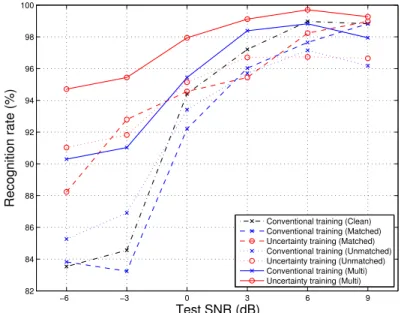
More detailed analysis is provided in Fig. 6, where the average accuracy resulting from the Wiener+VTS estimator together with uncertainty decoding is plotted as a function of the test SNR for all training strategies in all training conditions. Uncertainty training is shown to outperform conventional training for most test SNRs.

4.3. Results for other uncertainty estimators

The goal of the following experiment is to assess the results with different un-certainty estimators. To this aim, we compare the recognition accuracy resulting from the 9 uncertainty estimators in Section 4.1.4 for all training strategies in all training conditions.

Table 2 shows the average accuracies, where uncertainty decoding was per-formed in all cases. In all training conditions, the best results are obtained either by the Wiener+VTS estimator or by the Beta f+VTS estimator and, ac-cording to aχ2 _{test, these two estimators with uncertainty training are better} with 98% confidence level than all estimators with conventional training in the multi-condition case. Moreover, uncertainty training outperforms conventional training for each estimator, except for Beta+VTS and Beta f+VTS in matched or unmatched conditions, and on average over all estimators in all noisy condi-tions. These results further support the proposed uncertainty training approach and indicate that it is reasonably robust to the choice of the estimator. Note also that MM (unsc.) and MM (Gales) lead to similar performance, the for-mer being slightly better in almost all cases. The proposed Beta f estimator outperforms the conventional Beta estimator of Kolossa et al. (2010) only in combination with VTS. Finally, it should be noted that the recognition results are loosely correlated with the accuracy of the estimated MFCCs measured in Appendix E.2.

(17)

−6 −3 0 3 6 9 60 65 70 75 80 85 90 95 100 Test SNR (dB) Recognition rate (%)

Conventional training (Clean) Conventional training (Matched) Uncertainty training (Matched) Conventional training (Unmatched) Uncertainty training (Unmatched) Conventional training (Multi) Uncertainty training (Multi)

Figure 6: Average speaker recognition accuracy (in %) as a function of the test SNR for all training strategies in all training conditions with the Wiener+VTS uncertainty estimator. The results are averaged over the training SNRs corresponding to each training condition. Uncertainty decoding is performed in all cases.

All uncertainty estimators presented in Section 4.1.4 lead to full covariance matrices. Given that the GMM covariances are diagonal, considering diagonal uncertainty covariance matrices would significantly reduce the computational load. Thus, we also evaluate the 9 estimators with diagonal covariances ob-tained by simply setting to zero the off-diagonal elements of the full uncertainty covariance matrix estimators considered above. As shown in Table 3, using di-agonal uncertainty covariances leads to a systematic loss in recognition accuracy in a multi-condition setting. This clearly indicates that the correlation of errors between different feature dimensions is an important point that must be taken into account. Similar behaviour is observed in other training conditions.

4.4. Benchmarking results for oracle uncertainty estimators

In order to demonstrate that the proposed uncertainty training strategy will remain useful in the future even with improved uncertainty estimators, we redo the same experiments with two different oracle uncertainty estimators. By oracle, we mean that the optimal uncertainties are computed from the clean datayin the ML sense in a benchmarking context.

Deng et al. (2005) constrain the oracle uncertainty covariance to bediagonal. In this case the oracle uncertainty is given by ¯Σy,n= diag

[¯σy2,mn]m with

¯

(18)

Training

Uncertainty condition Clean Matched Unmatched Multi estimator Training

strategy Conv. Conv. Uncrt. Conv. Uncrt. Conv. Uncrt. Beta+MM (unsc.) 75.96 78.70 82.60 77.79 81.69 85.17 91.18 Beta f+MM (unsc.) 73.28 80.07 81.64 79.06 80.32 84.83 90.37 Wiener+MM (unsc.) 68.38 75.59 87.35 74.26 85.00 79.53 91.64 Beta+MM (Gales) 75.51 78.60 82.87 77.58 81.52 85.02 91.13 Beta f+MM (Gales) 72.70 79.88 81.32 78.84 80.26 84.73 90.39 Wiener+MM (Gales) 68.14 75.59 86.59 74.16 84.92 79.56 91.42 Beta+VTS 77.99 88.95 86.69 88.52 86.30 92.06 92.52 Beta f+VTS 81.37 90.15 88.80 89.65 87.98 92.38 93.80 Wiener+VTS 80.74 88.92 90.61 88.63 89.67 91.50 93.73 Average over all estimators 74.90 81.83 85.39 80.94 84.19 86.09 91.80

Table 2: Average speaker recognition accuracy (in %) for all training strategies in all training conditions as a function of 9 different uncertainty estimators with full covariance. Uncertainty decoding is performed in all cases.

Uncertainty

Uncertainty covariance Full Diagonal estimator Training

strategy Conv. Uncrt. Conv. Uncrt. Beta+MM (unsc.) 85.17 91.18 84.63 90.71 Beta f+MM (unsc.) 84.83 90.37 84.19 89.61 Wiener+MM (unsc.) 79.53 91.64 79.17 91.13 Beta+MM (Gales) 85.02 91.13 84.58 90.78 Beta f+MM (Gales) 84.73 90.39 84.22 89.80 Wiener+MM (Gales) 79.56 91.42 79.12 91.30 Beta+VTS 92.06 92.52 91.25 91.42 Beta f+VTS 92.38 93.80 90.76 91.96 Wiener+VTS 91.50 93.73 89.49 92.84

Average over all estimators 86.09 91.80 85.27 91.06

Table 3: Average speaker recognition accuracy (in %) for all training strategies as a function of 18 different uncertainty estimators, including 9 with full covariance and 9 with diagonal covariance. Multicondition training and uncertainty decoding are assumed in all cases.

We have found that relaxing this constraint leads to the new oracle estimator ¯

Σy,n= (¯yn−yn)(¯yn−yn)T, (23)

which is a full matrix of rank 1. This oraclerank-1estimator is more informative, since it encodes exactly the direction of the noise ¯yn−yn inRM and the only

remaining uncertainty is about its position on this line.

Table 4 reports the average speaker recognition accuracy for these two ora-cle estimators for all training strategies in all training conditions, in a similar way as the two bottom lines of Table 2. Naturally, the absolute scores in this ideal setting are always higher than in the previous setting. We see that uncer-tainty training outperforms conventional training in all cases and that the oracle rank-1 estimator achieves similar performance to conventional training on clean data. These results provide again a systematic confirmation of the superiority

(19)

of uncertainty training compared to conventional training and full uncertainty covariances compared to diagonal covariances.

Training

Oracle _condition Clean Matched Unmatched Multi

uncertainty _Training

estimator _strategy Conv. Conv. Uncrt. Conv. Uncrt. Conv. Uncrt.

diagonal 92.92 91.96 94.71 92.44 94.68 95.32 97.70

rank-1 99.66 96.10 99.46 96.37 99.36 98.75 99.68

Table 4: Average speaker recognition accuracy (in %) with uncertainty training and decoding for the two considered oracle uncertainty estimators.

For a closer look at the performance obtained with oracle uncertainty esti-mators, we display the results as a function of the test SNR in the same way as in Fig. 6. We only show the results for the diagonal estimator, since for the rank-1 estimator the results are very similar to each other and almost reach 100 % accuracy. It appears from Fig. 7 that the qualitative behaviour of these results is very similar to that of the blind estimator in Fig. 6. The absolute im-provement of uncertainty training over conventional training is naturally smaller in this oracle setting, but the relative improvement remains comparable.

−6 −3 0 3 6 9 82 84 86 88 90 92 94 96 98 100 Test SNR (dB) Recognition rate (%)

Conventional training (Clean) Conventional training (Matched) Uncertainty training (Matched) Conventional training (Unmatched) Uncertainty training (Unmatched) Conventional training (Multi) Uncertainty training (Multi)

Figure 7: Average speaker recognition accuracy (in %) as a function of the test SNR for all training strategies and training conditions with the oracle diagonal uncertainty estimator. The results are averaged over the training SNRs corresponding to each training condition. Uncertainty decoding is performed in all cases.

(20)

5. Conclusion

In this paper, we have argued that, when classifying noisy data, uncertainty should be taken into account both during training and decoding. We have intro-duced a new EM based technique that allows GMMs or HMMs to be trained on noisy data with dynamic Gaussian uncertainty and shown that it outperforms conventional training in both blind and oracle settings for a speaker recogni-tion task in a real-world multisource environment using a state-of-the-art signal enhancement front-end. Extensive evaluation has shown that this algorithm is robust to the training condition (matched, unmatched, or multicondition) and to the choice of the uncertainty estimator. The proposed algorithm performed best when used in conjunction with the VTS uncertainty propagation scheme fed with STFT-domain uncertainty estimates stemming from multichannel Wiener filtering.

As already mentioned, it is straightforward to extend this algorithm to the adaptation of acoustic models via, e.g., MAP or MLLR. Thus, it exhibits a great potential for other applications, such as noise-robust speaker diarization or automatic speech recognition. It is also particularly promising for a variety of Music Information Retrieval (MIR) tasks, e.g., singer identification within polyphonic music recordings, where the target sound source is never available in isolation so that clean training is impossible. Our approach is also not restricted to audio-related applications and can be applied for classification of other noise-corrupted data.

Rather than considering binary or Gaussian uncertainty, both the learning and decoding strategies could also be extended to other types of uncertainty models. For example, the uncertainty on each time frame could be encoded by some other kind of distribution, e.g., by a GMM.

Finally, since this study constitutes to the best of our knowledge the first use of VTS in the context of STFT-domain speech enhancement, it would be interesting to study its behavior more deeply, e.g., as a function of the SNR.

Appendix A. Derivation of the proposed uncertainty training algo-rithm

Let us consider A={¯y} as observed data, B={y,q} as latent data, and

(21)

log-likelihood of the complete data can be written as

−logp(¯y,y,q|θ) =−logp(¯y|y)−logp(y|q, θ)−logp(q|θ)

c =−logp(¯y|y) +1 2 X i,n δ(qn, i)log|Σi|+ (yn−µ_i)TΣ−_i1(yn−µ_i)−2 logωi =−logp(¯y|y) +1 2 X i,n {log|Σi|δ(qn, i)−2 logωiδ(qn, i) + trΣ−i1(ynynT−ynµT_i −µ_iy_nT+µ_iµT_i )δ(qn, i) =−logp(¯y|y) +1 2 X i,n

(log|Σi| −2 logωi)t0i,n

+ trΣ−1

i T2i,n−t1i,nµTi −µi(t1i,n)T+µiµTi t0i,n) (A.1)

with t0_i,n, t1

i,n and T2i,n defined by (12). This expression shows that the

log-likelihood of the complete data can be represented in the following form: logp(A,B|θ) =hη(θ),T(B)i+ν(θ) +φ(A,B), (A.2) whereT(B) is the vector of all scalar elements oft(B) =t0i,n,t1i,n,T2i,n _i,n,η(θ)

andν(θ) are some vector and scalar functions of the parametersθ, andφ(A,B) is a scalar function of the complete data. This means that the distribution of the complete data{p(A,B|θ)}θ belongs to theexponential family(Dempster et al.,

1977) and that the statistics t(B) are natural (sufficient) statistics (Ozerov et al., 2007) for this family. To derive an EM algorithm in this special case one needs to (i) maximize the likelihood of the complete data (thanks to (A.2) the ML solution can be always expressed as a function of the natural statistics

t(B)), and (ii) replace t(B) in the ML solution by its conditional expectation

ˆ_t₍A, θ′

),RBt(B)p(B|A, θ ′

)dBgiven the parametersθ′

estimated at the previous iteration.

It can be shown (e.g., by setting partial derivatives to zero) that the likeli-hood of the complete data (A.1) is maximized when

ωi= 1 N N X n=1 t0i,n, (A.3) µi= 1 PN n=1t0i,n N X n=1 t1 i,n, (A.4) Σi= 1 PN n=1t0i,n N X n=1 T2i,n−µiµTi . (A.5)

By computing the conditional expectations oft0

i,n,t1i,n andT2i,ngiven ¯yand

the previous parameter values θ′

(this computation relies on the conditional distribution of two Gaussian vectors as shown in Bishop (2006), Eqs. (2.81),

(22)

(2.82)), and by substituting them into (A.3), (A.4) and (A.5), we obtain the update equations of Algorithm 2.

Appendix B. Uncertainty training algorithm for HMMs

Let us consider aK-state HMM with continuous observation densities being

I-component GMMs (Rabiner, 1989), parametrized as

λ=n{πk}Kk=1,{akl}K,Kk,l=1,{µki,Σki, ωki}K,Ik,i=1

o

, (B.1)

where πk = P(s1 = k) and akl = P(sn+1 = k|sn = l) are, respectively,

ini-tial and transition probabilities, sn denotes the state at time n, and θk ,

{µ_ki,Σki, ωki}Ii=1 is thek-th state observation GMM specified as in (1). This kind of HMMs is commonly considered for automatic speech recognition. Algo-rithm 3 summarizes the EM updates for HMM training, analogous to those of Algorithm 2 for GMM training and developed under the same Gaussian uncer-tainty assumptions.

Appendix C. Estimation of the STFT-domain Wiener filter covari-ance with FASST

As mentioned in Section 4.1.2, both the mixture signals xf n and the

en-hanced target speech signals sf n considered in our experiments are binaural.

Denoting by ˜Σx,f n and ˜Σs,f n the respective prior covariance matrices of these

signals as estimated by FASST, the posterior mean and covariance of the mul-tichannel target are given by (see Bishop (2006), Eqs. (2.81), (2.82))

¯sf n = Σ˜s,f nΣ˜ −1 x,f nxf n, (C.1) ¯ Σs,f n = I−Σ˜s,f nΣ˜ −1 x,f n ˜ Σs,f n. (C.2)

As the first step towards MFCC extraction, the above signals are downmixed into single-channel mixturexf n and targetsf n signals as

xf n= 1 J X j x_{j,f n}, sf n= 1 J X j s_{j,f n}, (C.3)

wherej denotes the channel index andJ the number of channels (in our case

J = 2). The posterior mean and variance of the single-channel target are then derived as ¯ sf n= 1 J X j ¯ s_{j,f n}, σ¯2_s_{,f n}= 1 J2 X j,j′ ¯ Σs,f n[j, j′]. (C.4)

(23)

Appendix D. Vector Taylor series uncertainty estimator for MFCCs

DenotingF(·) to be the nonlinear transform used to compute a given feature vector (here MFCCs), VTS (Moreno et al., 1996) consists of linearizing this transform by its first-order vector Taylor expansion in the neighborhood of the source estimate ¯sn:

yn =F(sn)≈ F(¯sn) +JF(¯sn) (sn−¯sn), (D.1)

whereJF(¯sn) is the Jacobian matrix ofF(sn) computed in sn = ¯sn. This leads

to the following estimates of the noisy feature value ¯yn and its uncertainty

covariance ¯Σy,n, as propagated through this (now linear) transform:

¯

yn=F(¯sn), Σ¯y,n=JF(¯sn) ¯Σs,nJF(¯sn)T. (D.2)

In the case of MFCC, F(·) can be expressed as (see, e.g., (Adilo˘glu and Vincent, 2011))

yn =F(sn) =Dlog(M|sn|), (D.3)

where D is theM ×M DCT matrix, M is theM ×F matrix containing the

Mel filter coefficients, and| · |and log(·) are both element-wise operations. With these notations the Jacobian matrix appearing in (D.2) can be expressed as

JF(¯sn) =D M

M|¯sn|11×F

, (D.4)

where11×F is an 1×F vector of ones and the magnitude| · | and the division

are both element-wise operations.

Appendix E. Supplementary material and detailed results Appendix E.1. Signal enhancement results

To evaluate the effectiveness of the considered signal enhancement algorithm, we first evaluate speech source separation performance in terms of the SDR, ISR, SIR, and SAR metrics proposed in (Vincent et al., 2012). As suggested in (Ozerov et al., 2007), we compare these results to reference results obtained by so-called “do nothing separation”. These reference results are simply equal to the mixture divided by two, as we separate two sources (target speech and background). The average results over the test set are reported in Table E.5. We see that the considered signal enhancement algorithm improves all source separation metrics except the SAR9_{) w.r.t. “do nothing separation” for all} SNRs.

9

As the “do nothing separation” approach is a linear separation method, it does not intro-duce any artifacts (SAR = +∞_{), while the considered non-linear separation method does.}

(24)

SNR -6 dB -3 dB 0 dB 3 dB 6 dB 9 dB Avg. SDR (dB) 2.62 4.23 5.53 6.52 7.18 7.63 5.62 Source ISR (dB) 7.63 7.84 8.08 8.45 8.58 8.67 8.21 separation SIR (dB) 5.03 7.70 10.79 13.34 15.98 18.58 11.90 SAR (dB) 9.93 10.91 12.11 13.13 14.00 14.78 12.48 “Do nothing” SDR (dB) -0.90 1.30 3.02 4.26 5.04 5.50 3.04 separation ISR (dB) 5.62 5.78 5.89 5.95 5.99 6.00 5.87 (target = SIR (dB) -5.41 -2.54 0.31 3.26 6.18 9.16 1.83 1/2 mix) SAR (dB) +∞ +∞ +∞ +∞ +∞ +∞ +∞

Table E.5: Average source separation metrics for the target speech source over the test set.

Appendix E.2. Feature enhancement results

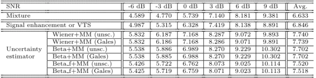
Here we evaluate whether the estimation of the conditional mean MFCCs can be improved by signal enhancement alone or whether it must be cascaded with uncertainty propagation. In order to evaluate the quality of feature en-hancement we use the Feature to Noise Ratio (FNR) measure we introduced in (Ozerov et al., 2011). The average results over the test set are reported in Table E.6. We see that signal enhancement slightly improves the FNR, except for high SNRs (6 and 9 dB), and that all the estimators improve the FNR over both the features computed from the mixture and those computed from the enhanced speech. SNR -6 dB -3 dB 0 dB 3 dB 6 dB 9 dB Avg. Mixture 4.589 4.770 5.739 7.140 8.181 9.381 6.633 Signal enhancement or VTS 4.987 5.315 6.328 7.419 8.138 8.891 6.846 Wiener+MM (unsc.) 5.832 6.187 7.168 8.287 9.072 9.893 7.740 Wiener+MM (Gales) 5.832 6.186 7.168 8.286 9.071 9.891 7.739 Uncertainty Beta+MM (unsc.) 5.538 5.886 6.989 8.270 9.229 10.302 7.702 estimator Beta+MM (Gales) 5.538 5.885 6.988 8.270 9.229 10.302 7.702 Beta f+MM (unsc.) 5.426 5.722 6.762 8.073 9.025 10.114 7.520 Beta f+MM (Gales) 5.425 5.719 6.759 8.071 9.023 10.113 7.518

Table E.6: Average FNR (dB) for the mean MFCC features of target speech over the test set. Note that, by definition of VTS, the mean features estimated by Wiener+VTS, Beta+VTS or Beta f+VTS are equal to those estimated from the enhanced speech signal without uncertainty propagation.

Appendix E.3. Detailed speaker recognition results

Table E.7 lists the speaker recognition results obtained for every consid-ered pair of training and test SNR conditions and for all training and decoding strategies with the Wiener+VTS uncertainty estimator. These detailed results correspond to the main average results reported in Table 1. One can note that in all the cases the best results lie usually near the diagonal of the 6×6 matrix corresponding to different training and test SNRs, i.e., the matched conditions.

(25)

Acknowledgments

The authors would like to thank Kamil Adilo˘glu for providing us with some parts of the necessary code for computing the MFCC uncertainty, Ram´on Fer-nandez Astudillo and Dorothea Kolossa for detailed explanation of their work, and the anonymous reviewers for their valuable comments.

References

Adilo˘glu, K., Vincent, E., 2011. An uncertainty estimation approach for the extraction of individual source features in multisource recordings. In: EU-SIPCO, 19th European Signal Processing Conference. pp. 1663–1667. Arberet, S., Ozerov, A., Bimbot, F., Gribonval, R., 2012. A tractable

frame-work for estimating and combining spectral source models for audio source separation. Signal Processing 92 (8), 1886–1901.

Astudillo, R. F., 2010. Integration of short-time Fourier domain speech enhance-ment and observation uncertainty techniques for robust automatic speech recognition. Ph.D. thesis, Technical University Berlin.

Barker, J., Vincent, E., Ma, N., Christensen, H., Green, P., 2013. The PASCAL CHiME speech separation and recognition challenge. Computer Speech and Language (this issue).

Barker, J. P., Cooke, M. P., Ellis, D. P. W., 2005. Decoding speech in the presence of other sources. Speech Communication 45 (1), 5–25.

Bishop, C. M., 2006. Pattern Recognition and Machine Learning. Springer. Cooke, M., Jun. 2001. Robust automatic speech recognition with missing and

unreliable acoustic data. Speech Communication 34 (3), 267–285.

Delcroix, M., Kinoshita, K., Nakatani, T., Araki, S., Ogawa, A., Hori, T., Watanabe, S., Fujimoto, M., Yoshioka, T., Oba, T., Kubo, Y., Souden, M., Hahm, S.-J., Nakamura, A., 2011. Speech recognition in the presence of highly non-stationary noise based on spatial, spectral and temporal speech/noise modeling combined with dynamic variance adaptation. In: Proc. 1st Int. Workshop on Machine Listening in Multisource Environments (CHiME). pp. 12–17.

Delcroix, M., Nakatani, T., Watanabe, S., 2009. Static and dynamic variance compensation for recognition of reverberant speech with dereverberation pre-processing. IEEE Transactions on Audio, Speech, and Language Processing 17 (2), 324–334.

Dempster, A. P., Laird, N. M., Rubin., D. B., 1977. Maximum likelihood from incomplete data via the EM algorithm. Journal of the Royal Statistical Soci-ety. Series B (Methodological) 39, 1–38.

(26)

Deng, L., Acero, A., Plumpe, M., Huang, X., 2000. Large vocabulary speech recognition under adverse acoustic environments. In: Proc. 6th Int. Conf. on Spoken Language Processing (ICSLP). pp. 806–809.

Deng, L., Droppo, J., Acero, A., 2005. Dynamic compensation of HMM vari-ances using the feature enhancement uncertainty computed from a parametric model of speech distortion. IEEE Transactions on Speech and Audio Process-ing 13 (3), 412–421.

Droppo, J., Acero, A., 2008. Environmental robustness. In: Benesty, J., Sondhi, M. M., Huang, Y. (Eds.), Handbook of Speech Processing. Springer, pp. 653– 680.

Ephraim, Y., 1992. Statistical-model-based speech enhancement systems. Pro-ceedings of the IEEE 80 (10), 1526–1555.

Fischer, S., Kammeyer, K.-D., 1997. Broadband beamforming with adaptive postfiltering for speech acquisition in noisy environments. In: IEEE Interna-tional Conference on Acoustics, Speech, and Signal Processing (ICASSP’97). Vol. 1. pp. 359–362.

Gales, M. J. F., September 1995. Model-based techniques for noise robust speech recognition. Ph.D. thesis, University of Cambridge, UK.

Gales, M. J. F., 2011. Model-based approaches to handling uncertainty. In: Kolossa, D., Haeb-Umbach, R. (Eds.), Robust Speech Recognition of Uncer-tain or Missing Data - Theory and Applications. Springer, Berlin, Germany, pp. 101–125.

Gauvain, J.-L., Lee, C.-H., 1994. Maximum a posteriori estimation for multi-variate Gaussian mixture observations of Markov chains. IEEE Transactions on Speech and Audio Processing 2 (2), 291–298.

Ghahramani, Z., Jordan, M., 1994. Supervised learning from incomplete data via an EM approach. In: Advance on Neural Information Processing Systems. pp. 120–127.

Grinstead, C. M., Snell, J. L., 1997. Introduction to probability, 2nd Edition. American Mathematical Society, Providence, RI.

Kolossa, D., Astudillo, R. F., Abad, A., Zeiler, S., Saeidi, R., Mowlaee, P., da Silva Neto, J., Martin, R., 2011. CHIME challenge: approaches to robustness using beamforming and uncertainty-of-observation techniques. In: Proc. 1st Int. Workshop on Machine Listening in Multisource Environments (CHiME). pp. 6–11.

Kolossa, D., Astudillo, R. F., Hoffmann, E., Orglmeister, R., 2010. Indepen-dent component analysis and time-frequency masking for speech recognition in multitalker conditions. EURASIP Journal on Audio, Speech, and Music Processing 2010, 1–14.

(27)

Leggetter, C., Woodland, P., 1995. Flexible speaker adaptation using maximum likelihood linear regression. In: ARPA Spoken Lang. Technol. Workshop. pp. 104–109.

Liao, H., Gales, M. J. F., 2007. Adaptive training with joint uncertainty decod-ing for robust recognition of noisy data. In: Proceeddecod-ings of the IEEE Interna-tional Conference on Acoustics, Speech, and Signal Processing (ICASSP’07). Vol. 4. pp. 389–392.

Moreno, P. J., Raj, B., Stern, R. M., 1996. A vector Taylor series approach for environment-independent speech recognition. In: IEEE International Confer-ence on Acoustics, Speech, and Signal Processing (ICASSP’96). Vol. 2. pp. 733 – 736.

Moreno-Torres, J. G., Raeder, T., Alaiz-Rodr´ıguez, R., Chawla, N. V., Herrera, F., January 2012. A unifying view on dataset shift in classification. Pattern Recognition 45 (1), 521–530.

Nadeu, C., Pach`es-Leal, P., Juang, B.-H., 1997. Filtering time sequences of spectral parameters for speech recognition. Speech Communication 22, 315– 332.

Ozerov, A., Lagrange, M., Vincent, E., September 2011. GMM-based classifica-tion from noisy features. In: Proc. 1st Int. Workshop on Machine Listening in Multisource Environments (CHiME). Florence, Italy, pp. 30–35.

Ozerov, A., Lagrange, M., Vincent, E., 2012a. Acoustic Model Uncertainty Learning Experimental Toolbox (AMULET).

URLhttp://bass-db.gforge.inria.fr/amulet/

Ozerov, A., Philippe, P., Bimbot, F., Gribonval, R., 2007. Adaptation of Bayesian models for single-channel source separation and its application to voice/music separation in popular songs. IEEE Trans. on Audio, Speech and Language Proc. 15 (5), 1564–1578.

Ozerov, A., Vincent, E., September 2011. Using the FASST source separation toolbox for noise robust speech recognition. In: Proc. 1st Int. Workshop on Machine Listening in Multisource Environments (CHiME). Florence, Italy, pp. 86–87.

Ozerov, A., Vincent, E., Bimbot, F., 2012b. A general flexible framework for the handling of prior information in audio source separation. IEEE Transactions on Audio, Speech and Language Processingss 20 (4), 1118–1133.

Rabiner, L., 1989. A tutorial on hidden Markov models and selected applications in speech recognition. Proceedings of the IEEE 77 (2), 257–286.

Reynolds, D., 1995. Large population speaker identification using clean and telephone speech. IEEE Signal Processing Letters 2 (3), 46–48.

(28)

Sanguinetti, G., Milo, M., Rattray, M., Lawrence, N. D., 2005. Accounting for probe-level noise in principal component analysis of microarray data. Bioin-formatics 21 (19), 3748–54.

Shao, Y., Srinivasan, S., Jin, Z., Wang, D., 2010. A computational auditory scene analysis system for speech segregation and robust speech recognition. Computer Speech & Language 24 (1), 77–93.

Slaney, M., 1998. Auditory toolbox version 2. Tech. rep., Interval Research Corporation.

Srinivasan, S., Wang, D., 2007. Transforming binary uncertainties for robust speech recognition. IEEE Transactions on Audio, Speech and Language Pro-cessing 15 (7), 2130–2140.

Vincent, E., Araki, S., Theis, F. J., Nolte, G., Bofill, P., Sawada, H., Ozerov, A., Gowreesunker, B. V., Lutter, D., Duong, N. Q. K., 2012. The signal separation evaluation campaign (2007–2010): Achievements and remaining challenges. Signal Processing 92 (8), 1928–1936.

Woolson, R. F., Clarke, W. R., 2002. Statistical Methods for the Analysis of Biomedical Data, 2nd Edition. Wiley-Interscience, New-York.

(29)

Algorithm 3One iteration of the proposed uncertainty training EM algorithm for HMM training from noisy data.

Notations: The following standard notations (Rabiner, 1989) are used for intermediate likelihoods and probabilities:

ξkl,n ∝αk,naklbl(¯yn+1)βl,n+1, and X k,lξkl,n = 1, (B.2) γki,n∝αk,nβk,nωkiN(¯yn|µki,Σki+ ¯Σy,n), and X k,iγki,n= 1, (B.3) ˆ yki,n=Wki,n(¯yn−µ_ki) +µ_ki, (B.4) b

Ryy,ki,n= ˆyki,nyˆki,nT + (I−Wki,n)Σki, (B.5)

where Wki,n=Σki Σki+ ¯Σy,n −1 , (B.6) bk(¯yn) = X iωkiN(¯yn|µki,Σki+ ¯Σy,n), (B.7)

and αk,n and βk,n are computed using the forward-backward procedure

(Ra-biner, 1989) applied to the observations likelihoods (B.7).

M step. Update HMM parameters:

πi= K X k=1 γki,1, aij= 1 PN−1 n=1 PK k=1γki,n N_X−1 n=1 ξij,n, (B.8) ωki= 1 N N X n=1 γki,n, µ_ki= _PN 1 n=1γki,n N X n=1 γki,nyˆki,n, (B.9) Σki= 1 PN n=1γki,n N X n=1 γki,nRbyy,ki,n−µkiµT_ki, (B.10)

and, in caseΣki is constrained to be diagonal, set its off-diagonal elements to

(30)

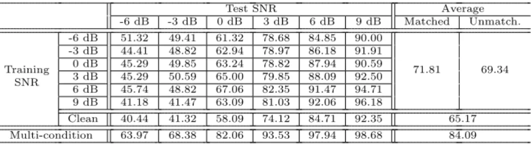
(A) Conventional training and decoding without signal enhancement Test SNR Average -6 dB -3 dB 0 dB 3 dB 6 dB 9 dB Matched Unmatch. -6 dB 51.32 49.41 61.32 78.68 84.85 90.00 -3 dB 44.41 48.82 62.94 78.97 86.18 91.91 0 dB 45.29 49.85 63.24 78.82 87.94 90.59 Training 3 dB 45.29 50.59 65.00 79.85 88.09 92.50 71.81 69.34 SNR 6 dB 45.74 48.82 67.06 82.35 91.47 94.71 9 dB 41.18 41.47 63.09 81.03 92.06 96.18 Clean 40.44 41.32 58.09 74.12 84.71 92.35 65.17 Multi-condition 63.97 68.38 82.06 93.53 97.94 98.68 84.09

(B)Conventional training / Conventional decoding with signal enhancement

Test SNR Average -6 dB -3 dB 0 dB 3 dB 6 dB 9 dB Matched Unmatch. -6 dB 62.35 68.09 79.71 89.26 91.76 93.53 -3 dB 61.32 69.41 79.41 89.56 91.03 93.38 0 dB 60.59 66.76 79.12 88.68 93.09 93.09 Training 3 dB 62.65 69.26 84.56 90.44 93.53 95.88 82.11 80.91 SNR 6 dB 58.24 64.41 82.06 92.21 93.68 96.62 9 dB 55.44 62.50 81.18 92.50 97.06 97.65 Clean 33.53 34.26 47.50 60.74 72.06 83.24 55.22 Multi-condition 74.41 82.21 90.59 96.62 98.24 98.68 90.12

(C)Conventional training / Uncertainty decoding with signal enhancement

(D)Uncertainty training / Uncertainty decoding with signal enhancement

Table E.7: Detailed speaker recognition accuracy (in %) for conventional vs. uncertainty training and decoding after signal enhancement. Both uncertainty training and decoding are based on the Wiener+VTS uncertainty estimator.