Int. J. Industrial Mathematics Vol. 1, No. 2 (2009) 135-145
A Direct Method for Numerically Solving
Integral Equations System Using Orthogonal
Triangular Functions
E. Baboliana, Z. Masourib, S. Hatamzadeh-Varmazyarc
(a) Department of Mathematics, Teacher Training University, Tehran, Iran (b) Department of Mathematics, Khorramabad Branch, Islamic Azad University,
Khorramabad, Iran
(c) Department of Electrical Engineering, Science and Research Branch, Islamic Azad University, Tehran, Iran
|||||||||||||||||||||||||||||||-Abstract
A practical direct method to compute numerical solutions of the linear Volterra and Fred-holm integral equations system is proposed. This approach is based on vector forms of triangular functions and its operational matrices and without any integration reduces an integral equations system to a system of algebraic equations. Numerical results of some examples show that the method is practical and has high accuracy.
Keywords: Integral equations system; Direct method; Vector forms; Triangular functions; Opera-tional matrix.
||||||||||||||||||||||||||||||||{
1 Introduction
Several methods for solving an integral equations system are presented. These methods often use a set of basis functions and obtain an approximate solution for these problems [1, 6, 7, 8].
In this paper, the ecient vector forms of triangular functions (TFs) proposed by Babolian et al. [2] are applied and a direct method for numerically solving the Volterra and Fredholm integral equations system is presented based on them. By using this method, a linear integral equations system can be easily reduced to a linear system of algebraic equations by just sampling of functions, multiplication and addition of matrices.
To make the article more readable, a brief description on the vector forms of the TFs and their properties is added.
Finally, the direct method using the orthogonal triangular basis functions will be used to solve some integral equations systems. The obtained results are compared with those of other methods. These comparisons show the eciency and accuracy of the current method to solve an integral equations system.
2 Review of vector forms of triangular functions
Triangular functions have been introuduced by Deb et al. [4] and studied and used by Babolian et al. [2] and Babolian et al. [3]. In this section, we review the vector forms of TFs vector forms and their properties proposed by Babolian et al. [2].
2.1 Denition and expansion
Two m-sets of triangular functions (TFs) are dened over the interval [0; T ) as [4]
T 1i(t) =
(
1 t ih
h ; ih 6 t < (i + 1)h;
0; otherwise;
T 2i(t) =
(
t ih
h ; ih 6 t < (i + 1)h;
0; otherwise;
(2.1)
where i = 0; 1; : : : ; m 1, with a positive integer value for m. Also, consider h = T=m, and T 1i as the ith left-handed triangular function and T 2i as the ith right-handed triangular
function. In this paper, it is assumed that T = 1, so TFs are dened over [0; 1), and h = 1=m.
Now, let T(t) be a 2m-vector dened as
T(t) = 0 @T1(t)
T2(t) 1
A ; 0 6 t < 1; (2.2)
where T1(t) and T2(t) are dened as follows:
T1(t) = [T 10(t); T 11(t); :::; T 1m 1(t)]T;
T2(t) = [T 20(t); T 21(t); :::; T 2m 1(t)]T;
(2.3)
in which T1(t) and T2(t) are called the left-handed triangular function (LHTF) vector and the right-handed triangular function (RHTF) vector, respectively.
Now, the expansion of any function f(t) with respect to TFs can be written as f(t) ' F 1TT1(t) + F 2TT2(t)
= FTT(t); (2.4)
where F 1 and F 2 are the coecients of TFs with F 1i= f(ih) and F 2i = f((i + 1)h), for
i = 0; 1; : : : ; m 1. Also, the 2m-vector F is dened as follows:
F = 0 @F 1
F 2 1
Now, assume that k(s; t) is a function of two variables. It can be expanded with respect to TFs as follows:
k(s; t) ' TT(s) K T(t); (2.6)
where T(s) and T(t) are 2m1- and 2m2- dimensional triangular functions and K is a
2m1 2m2 coecient matrix of TFs. For convenience, we put m1= m2= m. So, matrix
K can be written as
K = 0
@(K11)mm (K12)mm (K21)mm (K22)mm
1
A ; (2.7)
where K11, K12, K21, and K22 can be computed by sampling the function k(s; t) at points si and ti such that si= ti = ih, for i = 0; 1; : : : ; m. Therefore
(K11)i;j = k(si; tj); i = 0; 1; : : : ; m 1; j = 0; 1; : : : ; m 1;
(K12)i;j = k(si; tj); i = 0; 1; : : : ; m 1; j = 1; 2; : : : ; m;
(K21)i;j = k(si; tj); i = 1; 2; : : : ; m; j = 0; 1; : : : ; m 1;
(K22)i;j = k(si; tj); i = 1; 2; : : : ; m; j = 1; 2; : : : ; m:
(2.8)
2.2 Product properties
Let X be a 2m-vector which can be written as XT = (X1T X2T) such that X1 and X2
are m-vectors. Now, it can be concluded that
T(t)TT(t)X ' ~XT(t); (2.9)
where ~X = diag(X) is a 2m 2m diagonal matrix.
Now, let B be a 2m 2m matrix. So, it can be similarly concluded that
TT(t)BT(t) ' ^BTT(t); (2.10)
in which ^B is a 2m-vector with elements equal to the diagonal entries of matrix B. Also, Z 1
0 T(t)T
T(t) dt ' D; (2.11)
where D is the following 2m 2m matrix:
D = 0 @
h
3Imm h6Imm
h
6Imm h3Imm
1
A : (2.12)
2.3 Operational matrix
Expressing R0sT()d in terms of T(s), we can write Z s
0 T()d ' P T(s); (2.13)
where P2m2m, the operational matrix of T(s), is
P = 0
@P 1 P 2 P 1 P 2
1
where P 1 and P 2 are the operational matrices of integration of TFs as follows [4]
P 1 = h 2 0 B B B B B @
0 1 1 : : : 1 0 0 1 : : : 1 0 0 0 : : : 1 ... ... ... ... ... 0 0 0 : : : 0
1 C C C C C
A; P 2 = h 2 0 B B B B B @
1 1 1 : : : 1 0 1 1 : : : 1 0 0 1 : : : 1 ... ... ... ... ... 0 0 0 : : : 1
1 C C C C C
A: (2.15)
Now, the integral of any function f(t) can be approximated as Z s
0 f()d '
Z s
0 F
TT()d
' FTP T(s):
(2.16)
3 Numerical solutions of linear integral equations system
By using the results illustrated in the previous section about the TFs, a practical and accurate direct method for numerically solving integral equations system is proposed. Both Volterra and Fredholm systems can be solved by this method.
3.1 Fredholm integral equations system
Consider the following Fredholm integral equations system
fi(s) +
0 @Xn
j=1
j
Z b
a ki;j(s; t)xj(t)dt
1 A =Xn
j=1
jxj(s); for i = 1; 2; : : : ; n: (3.17)
In the above equations, the parameters j, the functions fi(s) and ki;j(s; t) are known and
xj(s), for j = 1; 2; : : : ; n are the unknown functions to be determined. Also, ki;j(s; t) 2
L2([0; 1) [0; 1)) and f
i(s); xj(s) 2 L2([0; 1)). Moreover, j 2 R, for j = 1; 2; : : : ; n, and
at least one of them is non-zero. Without loss of generality, it is supposed that a = 0 and b = 1, since any nite interval [a; b] can be transformed to interval [0; 1] by linear maps [5]. Approximating the functions fi(s), xj(s), and ki;j(s; t) with respect to TFs, (2.4) and
(2.6) give
fi(s) ' FiTT(s) = TT(s)Fi;
xj(s) ' XjTT(s) = TT(s)Xj;
ki;j(s; t) ' TT(s)Ki;jT(t);
(3.18)
where 2m-vectors Fi, Xj, and 2m 2m matrices Ki;j are TF coecients of fi(s), xj(s),
and ki;j(s; t), respectively. Note that Xj, for j = 1; 2; : : : ; n, are unknown vectors and
should be computed.
Substituting Eqs. (3.18) into (3.17) yields
FT
i T(s) ' n
X
j=1
jXjTT(s)
0 @Xn
j=1
jTT(s)Ki;j
Z 1
0 T(t)T T(t)X
jdt
1
Using Eq. (2.11) gives
TT(s)F
i' TT(s) n
X
j=1
jXj TT(s) n
X
j=1
jKi;jDXj: (3.20)
So,
Fi ' n
X
j=1
jXj n
X
j=1
jKi;jDXj: (3.21)
Now, replacing ' with = gives
n
X
j=1
(jI jKi;jD)Xj = Fi; for i = 1; 2; : : : ; n: (3.22)
System of equations (3.22) is a linear system of algebraic equations. In this system, jI jKi;jD, for i; j = 1; 2; : : : ; n are 2m2m matrices and Fis and Xjs are 2m-vectors.
So, xj(s) ' XjTT(s) are approximate solutions for Eqs. (3.17).
3.2 Volterra integral equations system
Consider the following linear Volterra integral equations system
fi(s) +
0 @Xn
j=1
j
Z s
0 ki;j(s; t)xj(t)dt
1 A =Xn
j=1
jxj(s); for i = 1; 2; : : : ; n; (3.23)
where the parameters j and the functions fi(s) and ki;j(s; t) are known functions, but
xj(s), for j = 1; 2; : : : ; n, are not. Also, ki;j(s; t) 2 L2([0; 1) [0; 1)) and fi(s); xj(s) 2
L2([0; 1)). Moreover, j 2 R, for j = 1; 2; : : : ; n, and at least one of them is non-zero.
Similar to the direct method for Fredholm integral equations system, substituting Eqs. (3.18) into (3.23) yields
FiTT(s) 'Xn
j=1
jXjTT(s)
0 @Xn
j=1
jTT(s)Ki;j
Z s
0 T(t)T T(t)X
jdt
1
A : (3.24)
Using Eq. (2.9) and the operational matrix P , in Eq. (2.13) gives
FiTT(s) '
n
X
j=1
jXjTT(s) n
X
j=1
jTT(s)Ki;jX~j
Z s
0 T(t)dt
'Xn
j=1
jXjTT(s) n
X
j=1
jTT(s)Ki;jX~jP T(s);
(3.25)
where Ki;jX~jP , for i; j = 1; 2; : : : ; n, are 2m 2m matrices. Using Eq. (2.10) gives
in which ^Xj, for j = 1; 2; : : : ; n, are 2m-vectors with components equal to the diagonal
entries of the matrices Ki;jX~jP .
Combining (3.25) and (3.26) gives
FT
i T(s) ' n
X
j=1
jXjTT(s) n
X
j=1
jX^jTT(s): (3.27)
Hence, replacing ' with = results in
n
X
j=1
(jXj jX^j) = Fi; for i = 1; 2; : : : ; n: (3.28)
System of equations (3.28) is a linear system of algebraic equations for the unknowns 2m-vectors Xj, for j = 1; 2; : : : ; n. So, approximate solutions xj(s) ' XjTT(s) can be
computed for Eq. (3.23) without using any projection method.
4 Numerical examples
In this section, some examples are investigated by the proposed method. Then, the nu-merical results obtained here are compared with the exact solutions and the approximate solutions obtained by the methods proposed in dierent references.
The computations associated with the examples have been performed using Matlab 7 on a Personal Computer.
Example 4.1. Consider the following Fredholm integral equations system [6, 7]: 8
> < > :
x1(s) +R01es t x1(t) dt +R01e(s+2)t x2(t) dt = 2es+es+1s+11;
x2(s) +R01est x1(t) dt +R01es+t x2(t) dt = es+ e s+es+1s+11;
(4.29)
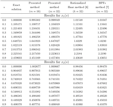
with the exact solutions x1(s) = es and x2(s) = e s. The numerical results are shown in
Table 1
Numerical results for Example 4.1
s Exact solution
Presented method (m = 16)
Presented method (m = 32)
Rationalized Haar method [6]
(k = 32)
BPFs method [7]
(m = 32) Results for x1(s)
0.0 1.000000 0.995382 0.998849 1.01548 1.01047 0.1 1.105171 1.100717 1.104019 1.11531 1.11641 0.2 1.221403 1.216431 1.220211 1.22495 1.22496 0.3 1.349859 1.344486 1.348574 1.34538 1.34547 0.4 1.491825 1.486258 1.490378 1.47764 1.47776 0.5 1.648721 1.641923 1.647027 1.6229 1.6230 0.6 1.822119 1.815578 1.820420 1.83904 1.83910 0.7 2.013753 2.006342 2.011984 2.01983 2.01982 0.8 2.225541 2.217450 2.223613 2.2184 2.2190 0.9 2.459603 2.451169 2.457404 2.43648 2.43651
Results for x2(s)
0.0 1.000000 1.002677 1.000667 0.98456 0.98470 0.1 0.904837 0.907913 0.905568 0.89646 0.89657 0.2 0.818731 0.821581 0.819474 0.81625 0.81636 0.3 0.740818 0.743565 0.741531 0.74322 0.74351 0.4 0.670320 0.673023 0.670969 0.67673 0.67682 0.5 0.606531 0.608759 0.607086 0.61619 0.61621 0.6 0.548812 0.551082 0.549356 0.54382 0.54386 0.7 0.496585 0.498480 0.497077 0.49518 0.49520 0.8 0.449329 0.450876 0.449731 0.45091 0.45010 0.9 0.406570 0.407751 0.406848 0.41060 0.41070 Example 4.2. For the following linear Fredholm integral equations system [1]:
8 > < > :
x1(s) R01 s+t3 (x1(t) + x2(t)) dt = 18s + 1736;
x2(s) R01st (x1(t) + x2(t)) dt = s2 1912s + 1;
(4.30)
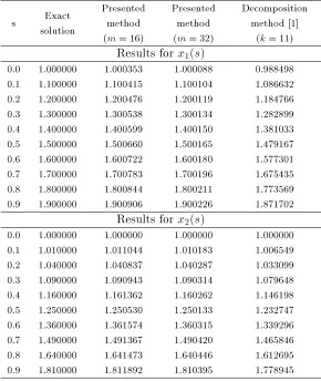
with the exact solutions x1(s) = s + 1 and x2(s) = s2+ 1, Table 2 shows the numerical
Table 2
Numerical results for Example 4.2
s Exact solution
Presented method (m = 16)
Presented method (m = 32)
Decomposition method [1]
(k = 11) Results for x1(s)
0.0 1.000000 1.000353 1.000088 0.988498 0.1 1.100000 1.100415 1.100104 1.086632 0.2 1.200000 1.200476 1.200119 1.184766 0.3 1.300000 1.300538 1.300134 1.282899 0.4 1.400000 1.400599 1.400150 1.381033 0.5 1.500000 1.500660 1.500165 1.479167 0.6 1.600000 1.600722 1.600180 1.577301 0.7 1.700000 1.700783 1.700196 1.675435 0.8 1.800000 1.800844 1.800211 1.773569 0.9 1.900000 1.900906 1.900226 1.871702
Results for x2(s)
0.0 1.000000 1.000000 1.000000 1.000000 0.1 1.010000 1.011044 1.010183 1.006549 0.2 1.040000 1.040837 1.040287 1.033099 0.3 1.090000 1.090943 1.090314 1.079648 0.4 1.160000 1.161362 1.160262 1.146198 0.5 1.250000 1.250530 1.250133 1.232747 0.6 1.360000 1.361574 1.360315 1.339296 0.7 1.490000 1.491367 1.490420 1.465846 0.8 1.640000 1.641473 1.640446 1.612695 0.9 1.810000 1.811892 1.810395 1.778945
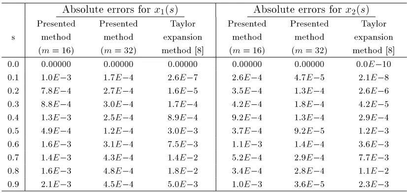
Example 4.3. For the following linear Volterra integral equations system [8]: 8
> < > :
x1(s) R0s(s t)3 x1(t) dt R0s(s t)2 x2(t) dt = y1(s);
x2(s) R0s(s t)4 x1(t) dt R0s(s t)3 x2(t) dt = y2(s);
(4.31)
y1(s) and y2(s) are chosen such that the exact solutions are x1(s) = s2+ 1 and x2(s) =
Table 3
Numerical results for Example 4.3
Absolute errors for x1(s) Absolute errors for x2(s)
s
Presented method (m = 16)
Presented method (m = 32)
Taylor expansion method [8]
Presented method (m = 16)
Presented method (m = 32)
Taylor expansion method [8] 0.0 0.00000 0.00000 0.00000 0.00000 0.00000 0.0E 10
0.1 1.0E 3 1.7E 4 2.6E 7 2.6E 4 4.7E 5 2.1E 8
0.2 7.8E 4 2.7E 4 1.6E 5 3.5E 4 1.3E 4 2.6E 6
0.3 8.8E 4 3.0E 4 1.7E 4 4.2E 4 1.8E 4 4.2E 5
0.4 1.3E 3 2.5E 4 8.9E 4 9.2E 4 1.3E 4 2.9E 4
0.5 4.9E 4 1.2E 4 3.0E 3 3.7E 4 9.2E 5 1.2E 3
0.6 1.6E 3 3.1E 4 7.5E 3 1.1E 3 1.4E 4 3.6E 3
0.7 1.4E 3 4.3E 4 1.4E 2 5.2E 4 2.9E 4 7.7E 3
0.8 1.6E 3 4.8E 4 1.8E 2 3.4E 4 2.8E 4 1.1E 2
0.9 2.1E 3 4.5E 4 5.0E 3 1.0E 3 3.6E 5 2.3E 3
5 Error evaluation
The direct method based on TFs and its operational matrix transforms, without applying any projection method, a nonlinear Volterra or Fredholm integral equations system to a set of algebraic equations. Its applicability and accuracy were checked on three examples. In these examples the approximate solution is briey compared with the exact and ap-proximate solutions obtained by the methods proposed in [1, 6, 7, 8]. It follows from the numerical results that the accuracy of the solutions obtained using the TFs is quite satis-factory in comparison with the other methods. The methods presented in [6, 7]. use the block-pulse and rationalized Haar functions, respectively, to obtain the numerical solutions of the integral equations system given in Example (4.1). Comparing the results presented in Table 1 shows that our method is more accurate and the number of its calculations is smaller. Also, [1] proposes the decomposition method to solve the problem presented in Example (4.2). It seems that the direct method is more accurate and practical than the decomposition method. Furthermore, the number of calculations of the direct method is smaller. As regards Example (4.3), [8] presents the Taylor expansion method. This method reduces the system of integral equations to a linear system of ordinary dierential equations. After constructing boundary conditions, this system reduces to a system of equations. Although the results included in Table 3 do not show the categorical superi-ority of the proposed method over the Taylor expansion method from the viewpoint of accuracy, it seems that the number of calculations in the direct method is considerably smaller than that of the Taylor expansion method. This is due to the fact that the gen-eration of the algebraic equations system in the current method needs just sampling of functions, multiplication and addition of matrices, and needs no integration.
To show the convergence and stability of this approach, the mean-absolute errors at the points s in Tables 1-3 are computed for dierent values of m.
Consider the mean-absolute error as follows
Em n;j = n1
n
X
i=1
where xj(si) and xjm(si) are the jth exact and approximate solutions at points si,
respec-tively.
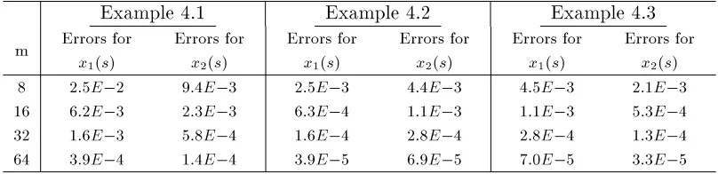
For Examples (4.1), (4.2), (4.3), these errors for ten points s = 0; 0:1; 0:2; : : : ; 0:9 and m = 8; 16; 32; 64 are illustrated in Table 4.
Table 4
Mean-absolute errors for Examples (4.1, 4.2, 4.3)
Example 4.1 Example 4.2 Example 4.3
m Errors for x1(s)
Errors for x2(s)
Errors for x1(s)
Errors for x2(s)
Errors for x1(s)
Errors for x2(s)
8 2.5E 2 9.4E 3 2.5E 3 4.4E 3 4.5E 3 2.1E 3
16 6.2E 3 2.3E 3 6.3E 4 1.1E 3 1.1E 3 5.3E 4
32 1.6E 3 5.8E 4 1.6E 4 2.8E 4 2.8E 4 1.3E 4
64 3.9E 4 1.4E 4 3.9E 5 6.9E 5 7.0E 5 3.3E 5
These results show that by increasing the number of TFs over [0; 1), the error of the method decreases rapidly. This conrms the direct method proposed in this article has convergence and stability. So, one can run the method by increasing m until the computed results have an appropriate accuracy.
6 Conclusion
This article introduced a numerical method to solve the linear Volterra and Fredholm integral equations system. Using vector forms of TFs, and the operational matrix of integration, this approach transforms an integral equations system to a system of algebraic equations directly.
The benets of this method are the low cost of setting up the equations without applying any projection methods such as the Galerkin or the collocation methods, and using no integration to approximate the functions. So, this method may be run very quickly even for large values of m.
Finally, the numerical results have very good accuracy and show that the proposed method is practical.
References
[1] E. Babolian, J. Biazar, A.R. Vahidi, The decomposition method applied to systems of Fredholm integral equations of the second kind, Appl. Math. Comput. 148 (2004) 443-452.
[2] E. Babolian, Z. Masouri, S. Hatamzadeh-Varmazyar, Numerical solution of nonlinear Volterra-Fredholm integro-dierential equations via direct method using triangular functions, Computers and Mathematics with Applications, 58 (2009) 239-247. [3] E. Babolian, R. Mokhtari, M. Salmani, Using direct method for solving variational
[4] A. Deb, A. Dasgupta, G. Sarkar, A new set of orthogonal functions and its application to the analysis of dynamic systems, Journal of the Franklin Institute, 343 (2006) 1-26. [5] L.M. Delves, J.L. Mohamed, Computational methods for integral equations,
Cam-bridge University Press, CamCam-bridge, 1985.
[6] K. Maleknejad, F. Mirzaee, Numerical solution of linear Fredholm integral equations system by rationalized Haar functions method, Intern. J. Computer Math. 80 (2003) 1397-1405.
[7] K. Maleknejad, M. Shahrezaee, H. Khatami, Numerical solution of integral equations system of the second kind by Block-Pulse functions, Appl. Math. Comput. 166 (2005) 15-24.