RESEARCH NOTE
EXPERIMENTAL ANALYSIS FOR MEASURING ERRORS IN
WHEELED MOBILE ROBOTS
M. H. Korayem, T. Bani Rostam
Robotic Research Laboratory, College of Mechanical Engineering, Iran University of Science and Technology, Tehran, Iran,
[email protected] , [email protected]
(Received: Aug 28, 2004– Accepted in Revised Form: Aug. 5, 2005)
Abstract This paper presents experimental analysis of wheeled mobile robots.
Mathematical modelling of the mobile robot is presented. The mobile robots consist of an omni-directional and three differential drive mobile robots are tested and moved in given trajectories and the systematic errors of the robots are determined. A new method for omni-direction mobile robot was introduced in which the robot was programmed to move in direction of each wheel shaft. Finally, the mobile robot is moved in given trajectories and the systematic errors of the robot are determined.
Keywords Measurement, Mobile robot, Test, Experimental Analysis.
ﺪﻴﻜﭼ ﻩ
ﻭﺕﺎـﺑﺭﺖـﮐﺮﺣﺮـﺑﻞـﻣﺍﻮﻋﺯﺍﮏـﻳﺮـﻫﺮﻴﺛﺎﺗ،ﺎﻄﺧﻩﺪﻧﺭﻭﺁﺩﻮﺟﻭﻪﺑﻞﻣﺍﻮﻋ،ﮎﺮﺤﺘﻣﺕﺎﺑﺭﻱﺎﻫﺎﻄﺧﻪﻟﺎﻘﻣﻦﻳﺍﺭﺩ
ﺵﻭﺭ
ﻲـﻣﺭﺍﺮـﻗﻲـﺳﺭﺮﺑﺩﺭﻮـﻣﮎﺮـﺤﺘﻣﺕﺎـﺑﺭﯽﺘﮐﺮﺣﯼﺎﻫﺎﻄﺧﺡﻼﺻﺍﯼﺎﻫ ﺩﺮـﻴﮔ
.
ﺘﺴـﻴﺳﻱﺎـﻫﺎﻄﺧﺭﻮـﻈﻨﻣﻦﻳﺪـﺑ ﻭﮏﻴﺗﺎﻤ
ﻲﻣﻪﺒﺳﺎﺤﻣﻲﻠﺻﺍﺖﻴﻌﻗﻮﻣﺯﺍﺕﺎﺑﺭﻑﺍﺮﺤﻧﺍﻩﺯﺍﺪﻧﺍﻭﺎﻬﻧﺁﺯﺍﮏﻳﺮﻫﺩﺎﺠﻳﺍﻞﻣﺍﻮﻋ،ﻩﺪﺷﻲﺳﺭﺮﺑ،ﮏﻴﺗﺎﻤﺘﺴﻴﺳﺮﻴﻏ
ﺩﻮﺷ
. ﺭﻮـﻈﻨﻣﻪﺑ
ﻪﻴﺒﺷﺭﺩﺮﺛﻮﻣﻱﺎﻫﺮﺘﻣﺍﺭﺎﭘ،ﻩﺪﺷﻱﺯﺎﺳﻪﻴﺒﺷﻲﻠﺿﺎﻔﺗﺥﺮﭼﮎﺮﺤﺘﻣﺕﺎﺑﺭﺖﮐﺮﺣﻉﻮﺿﻮﻣﺮﺘﺘﺣﺍﺭﻭﻖﻴﻗﺩﻲﺳﺭﺮﺑ
ﺞﻳﺎﺘﻧﻭﯼﺯﺎﺳ
ﻲﻣﻲﺑﺎﻳﺯﺭﺍﻥﺁﺯﺍﻞﺻﺎﺣ ﺩﺩﺮﮔ
.
ﻨﻣﻪﺑ ﺖﺴﺗﺕﺎﺑﺭﻲﺗﺎﺸﻳﺎﻣﺯﺁﺯﺍﻩﺩﺎﻔﺘﺳﺍﺎﺑﮎﺮﺤﺘﻣﺕﺎﺑﺭﺭﺩﺩﻮﺟﻮﻣﻱﺎﻫﺎﻄﺧﻥﺩﻮﻤﻧﻑﺮﻃﺮﺑﺭﻮﻈ
ﻲﻣﻪﺒﺳﺎﺤﻣﺢﻴﺤﺼﺗﺐﻳﺍﺮﺿﺲﭙﺳﻭﺎﻄﺧﺭﺍﺪﻘﻣ،ﺕﺎﺸﻳﺎﻣﺯﺁﺞﻳﺎﺘﻧﺯﺍﻩﺩﺎﻔﺘﺳﺍﺎﺑ،ﻩﺪﺷ
ﻮﺷ ﻧﺪ
. ﻭﺢﻴﺤﺼـﺗﺐﻳﺍﺮـﺿﺯﺍﻩﺩﺎﻔﺘـﺳﺍﺎﺑ
ﺕﺎﺑﺭﺭﺎﺘﺧﺎﺳﺭﺩﻥﺁﻝﺎﻤﻋﺍ ،
ﺿﻝﺎﻤﻋﺍﺎﺑٌﺍﺩﺪﺠﻣﺕﺎﺸﻳﺎﻣﺯﺁﻭﻩﺪﺷﺢﻴﺤﺼﺗﺕﺎﺑﺭﺖﮐﺮﺣ
ﻲـﻣﺭﺍﺮـﮑﺗﺢﻴﺤﺼـﺗﺐﻳﺍﺮ ﺩﺩﺮـﮔ
. ﺞﻳﺎـﺘﻧ
ﻲﻣﻪﺴﻳﺎﻘﻣ،ﻩﺪﺷﯽﺳﺭﺮﺑ،ﺕﺎﺑﺭﺩﺮﮑﻠﻤﻋﻭﺢﻴﺤﺼﺗﺐﻳﺍﺮﺿﺮﻴﺛﺎﺗﺩﺭﻭﺁﺮﺑﺖﻬﺟﺭﻮﮐﺬﻣﺕﺎﺸﻳﺎﻣﺯﺁﺯﺍﻞﺻﺎﺣ
ﺩﺩﺮﮔ
. ﺭﻮﮐﺬـﻣﺩﺭﺍﻮـﻣ
ﺕﺎﺑﺭﻪﺳﺩﺭﻮﻣﺭﺩ ﺖـﺳﺍﻩﺪﻳﺩﺮﮔﻪﺋﺍﺭﺍﻞﺻﺎﺣﺞﻳﺎﺘﻧﻭﻡﺎﺠﻧﺍﻱﺪﺋﻮﺳﺥﺮﭼﻪﺳﺕﺎﺑﺭﮏﻳﻭﻲﻠﺿﺎﻔﺗﺥﺮﭼ
. ﺭﻮـﻈﻨﻣﻪـﺑﻦﻴـﻨﭽﻤﻫ
ﻖﻴﻗﺩﻲﺳﺭﺮﺑ
ﺮﺗ ﺕﺎﺑﺭﺯﺍﮏﻳﺮﻫﺖﮐﺮﺣ،ﻉﻮﺿﻮﻣ
ﺎـﺑﺎـﻄﺧﺯﻭﺮـﺑﻝﺎـﻤﺘﺣﺍ،ﻪﺘﻓﺮﮔﺭﺍﺮﻗﻪﺴﻳﺎﻘﻣﺩﺭﻮﻣﻝﺎﻣﺮﻧﻊﻳﺯﻮﺗﺯﺍﻩﺩﺎﻔﺘﺳﺍﺎﺑﺎﻫ
ﺖﮐﺮﺣﺭﺩﻒﻠﺘﺨﻣﺮﻳﺩﺎﻘﻣ ﻲﻣﺩﺭﻭﺁﺮﺑﺕﺎﺑﺭﯼﺪﻌﺑﻱﺎﻫ
ﺩﺩﺮﮔ
.
1. INTRODUCTION
Interested researches on mobile robots have been increased in the past few years [1]. Some
researchers have considered slipping motion between the wheels and motion surface in mobile robots and vehicles. Choi and Sreenivasan have designed articulated wheeled vehicles with
wheels, considering kinematics only [4]. Balakrishna and Ghosal developed a traction model accounting for slip in non-holonomic wheeled mobile robots [5]. Scheding et al. present experimental evaluation of a navigation system that handles autonomous vehicle wheel slip [6]. Watanabe et al. designed a controller for an autonomous omni-directional mobile robot for service applications [7]. Dickerson and Lapin present a controller for omni-directional Sweden- wheeled vehicles that includes wheel slip detection and compensation [8].
Cybermotion K2A utilises synchronize-drive, which makes it insensitive to non-systematic errors. CLAPPER, consisted of two TRC Lab Mates connected by a compliant linkage, uses two rotary encoders to measure the rotation of the lab mates relative to the compliant linkage, and a linear encoder to measure the relative distance between their centre points, giving it the unique ability to measure and correct non-systematic dead reckoning errors during motion [9].
This paper presents design a model for four mobile robots including an omni-directional mobile robot and three differential drive robots. The research is concluded with experimental tests in order to determine and correct the systematic errors of the robots with using UMBmark test and a new method. Finally, the results are comparing with statistical analysis.
2. DESIGN OF MOBILE ROBOTS
For designing a robot some factors such as: robot’s job environment and robot’s tasks play an important role. In addition other factors such as: weight of robot, type of wheels, material of wheels and rollers and control devices influence in design. Design process starts by knowledge of robot parts and environment.
2.1. Omni-Directional three-wheeled Robot
The structure of this robot consists of a computer controller, three DC motors with its own drivers and incremental encoders for each drive wheel are shown in Figureure. 1. The mechanical parts and manufactured wheels of robot are consisted of a central plane with eight rollers and schematic view of them [10-11].
Figureure 1. .Manufactured Omni-directional robot
One Microcontroller (89C51) controls the wheels speed. Sensors obtain environment data and transmit it to processor. After data processing by microprocessor, commands are sent to microcontroller and it translates and transmits them to DC motors. In addition, vision system provides data from physical obstacles and their distance. The robot control algorithm is shown in Figureure. 2. This design has capability of adding new sensors for different aims.
2.2. Differential Drive Robot
The construction of differential drive robot is consisting of two drive wheels and two castor wheels, two pulley-belt systems, two shafts that connect the wheels to pulleys, a small driver system with L297 IC and a processor for data processing transmitted to the robot.
Case I: Robotest
Robotest consists of two drive wheels with its own stepper that is controlled by a Pentium III computer and two free castor wheels providing the robot stability. The castors cause slipping during direction changes. These parts are shown in manufactured model of the robot as shown in Figureure. 4.
Case II:MoboLab
This robot named MoboLab has dimension of
20 60
60× × 3
cm
and weighs of 10 kg.(Figureure. 5) Mobolab has two drive wheels and two free castor wheels, two stepping motors with a
78/16 spurgears transmission ratio for each motor and a maximum 1 N.m output. The motor shaft rotates
1
.
8
o per step.The rotation can be transformed to a linear movement of wheels that depends on the diameters of the gear and wheels. The diameter of driver wheels is about 100 mm and the width is about 30 mm. The material of wheels is rubber in the contact point with ground. There is a little elastic deformation in the gears.
The controller computes the command signals from the reference trajectory, processed by the sensory feedback measurement. For these purpose two shaft encoders are used. The controller communicates the command signals to pulse the stepper motor in the robot drive. The robot employs infrared sensor for obstacle avoidance and a 486-laptop computer for control and programming [12].
Figureure 5. Manufactured Mobolab (Case II)
Case III: Sweeper
This mobile robot is designed and constructed for sweeper robots competition and has two drive wheels, two castor wheels and two stepping motors (1.8 deg/step) with a spur gears transmission ratio. The diameter of drive wheels is about 195 mm and the thickness is about 10 mm. The material of wheels in contact point with ground is a rubber ring. This mobile manipulator has two arms that one of them is fixed to robot and the other rotate around it’s joint. Therefore this robot has three degrees of freedom comprising two DOF in base and one DOF in arm.
A Pentium III, 850 MHz processor is used for path detection algorithm processing. A webcam provides images acquisition from environment. With the data sent by camera, robot is able to detect the objects such as obstacles. This camera obtains environment data and sends it to microcontrollers and processor. After data processing by microprocessor, commands in packets are sent to microcontrollers through serial port, translated and finally transmit them to two stepper motors for moving and three motors for controlling the arms.
Figureure 6. Manufactured differential
3. KINEMATICS MODELLING OF MOBILE ROBOT
In this model we engage with a special condition that is called “Redundancy”. In this condition we must create some additional constraints for solving the kinematics and dynamic equations. Some of these constrains are obtained from non-slipping assumption and others are created by considering the logical and sufficient constraint in robot motion. In mobile robots these additional redundancy constraints may be functions of a special trajectory such as time. It is necessary to calculate the parameters that play a role in robot and are mandatory for obtaining the dynamic equation [11].
3.1. Omni-Directional Robot
The mobile frame T
M
M
y
x
,
]
[
is located at the centre of gravity of the robot. It is simple to compute the necessary wheel speed for a desired Cartesian velocity. It can be calculated from transformation matrixes, obtained from Denavit-Hartenberg notations.⎥
⎥
⎥
⎦
⎤
⎢
⎢
⎢
⎣
⎡
=
φ
θ
φ
θ
φ
ω
cos
sin
&
&
&
wheel (1)
Equation (1) shows the velocity matrixes which are calculated from angular and linear velocities Equations. The inverse kinematics equations can be calculated too [13].
3.2. Differential Drive Robots
According to the angular and linear velocities Equations, the linear and angular velocity of wheels (Eq. 2) and that of the base of robot (Eq. 3) are calculated by:
⎥ ⎥ ⎥ ⎦ ⎤ ⎢ ⎢ ⎢ ⎣ ⎡ + − + − + + + + + − − + + + = ϖ φ θ θ α θ α φ θ θ α θ α φ θ θ α θ α r l y x l y x r y x vWheel sin ] ) cos( ) sin( [ cos ] ) cos( ) sin( [ cos ) ( ) sin( ) cos( & & & & & & & & & ⎥ ⎥ ⎥ ⎦ ⎤ ⎢ ⎢ ⎢ ⎣ ⎡ =
φ
θ
φ
θ
ϖ
ω
cos sin & &Wheel (2)
⎥
⎥
⎥
⎦
⎤
⎢
⎢
⎢
⎣
⎡
+
−
+
=
0
cos
sin
sin
cos
θ
θ
θ
θ
y
x
y
x
v
Base&
&
&
&
,⎥
⎥
⎥
⎦
⎤
⎢
⎢
⎢
⎣
⎡
=
ϖ
ω
0
0
Base (3)
To get the robot position and orientation, Eq. (3) should satisfy the nonholonomic constraint [11]. The robot kinematics associated with the Jacobian matrix and velocity is defined by:
⎥ ⎥ ⎥ ⎦ ⎤ ⎢ ⎢ ⎢ ⎣ ⎡ ⎥ ⎥ ⎦ ⎤ ⎢ ⎢ ⎣ ⎡ − − − − − + − + = ⎥ ⎦ ⎤ ⎢ ⎣ ⎡
ω
π
θ
π
θ
π
θ
π
θ
ω
ω
y x l l r R L & & ) 2 sin( ) 2 cos( ) 2 sin( ) 2 cos( 1 (4) whereω
R andω
L are related to the angular velocity of robot wheels.4. DYNAMIC MODELLING OF MOBILE ROBOTS
The derivation began using the Lagrangian approach.The inverse kinematics equations for the mobile robot are as below: [11]
4.1. Omni-Directional Robot
Substituting the kinetic and potential terms into Lagrangian approach the equations of motion in the standard format are derived. The torques are influenced by the effect of potential and energy terms and calculated from solving these equations using in Maple software [10].
4.2. Differential Drive Mobile Robot
Consider the differential drive mobile robot, τ1/2 is the torque exerted on the robot by right or left wheel, and l is the distance between the centre of
gravity and the wheels. The actuator torques is calculated by solving the dynamic equations [10].
5. SIMULATION OF MOBILE ROBOT
It is possible to simulate the system kinematics and dynamic using Working Model and Visual Nastran soft wares for a given equations of motion. The
responses of the system to a simple-step input by maintaining the base in a fixed position (0o) are presented. This simulation deals only with mechanical factors (weight, inertia, etc.) and ignores any electrical components. Also these models do not consider any slippage occurred.
5.1. Omni-Directional Three-wheeled Robot
Figureure. 7 presents the robot modelled in Visual Nastran. The comparison of position and torques of motors 1, 2 and 3 between two simulating soft wares, Maple and Working Model, are presented elsewhere [10].
5.2. Differential Drive robots (Case I, II and III)
In this stage the robot modelled in Working Model is rotated around its axis. Because the low structural difference between three differential drive robots (case I, II and III) leads us to create
the same model for three robots. The additional objects such as motors are not shown. Figureure. 8 presents the model of robot drawn in Mechanical Desktop software and analysed in Working Model.
Figureure 7. The schematic model of three wheeled Figureure 8. The schematic model of
differentialomni-directional robot drive robot
Data acquired shows that the maximum amplitude of motion is approximately 6.35% for the X direction and 2.1% for the Y direction. The torque of motors 2 is depicted in Figureure. 9. As shown the predicted torques in Working Model has some difference with desired condition [13].
The source of these errors is that in theoretical models the friction is negligible but in Working Model and manufactured plans the friction plays an essential role. In this model the coefficient of friction is considered too large therefore the simulation have jumps with high amplitude.
6. EXPERIMENTAL TEST
Odometry is the measurement of the wheel rotation as a function of time. If the drive wheels of the robot are joined to a common axle, the position and orientation of the axle centre relative to the previous position and orientation can be determined from odometry measurements on all
wheels. In experimental tests, incremental encoders are mounted onto drive wheels.
6.1. Omni-directional Mobile Robot
For testing the omni-directional mobile robot a simple method was selected. This method is moving the robot in special trajectories such as in straight or in self-rotational paths. In this section the results of test in some trajectories are shown. The test was carried out ten times for a given trajectory and the systematic errors of robot are calculated by the inverse kinematics equations. Figureure. 10 shows the result of the path where the third wheel does not have angular velocity. The points show the final location of robot’s centre of gravity in working plane. In next test the second wheel has no angular velocity. Figureure 11 shows the result of this condition. Finally the first wheel with no angular velocity is considered (Figureure. 12). In all of these Figureures, the points are the final position of robot where it is stopped. The difference between final position of robot before and after calibration shows the effectiveness of process.
-90 -80 -70 -60 -50 -40 -30 -20 -10 0
0 1 2 3 4 5 6 7 8 9 10
Time [sec]
Torque
[N
.mm]
Maple
Working Model
-150 -100 -50 0 50 100 150 200 250
1200 1250 1300 1350 1400 1450 1500 1550 1600
Y [mm]
X [mm]
Before Calibration
After Calibration
Figureure 10. The robot moves parallel of third shaft
-100 -50 0 50 100 150 200 250 300
1300 1350 1400 1450 1500 1550 1600
Y [mm]
X [mm]
Before Calibration
After Calibration
6.2. Differential Drive Mobile Robot
6.2.1. Investigation of error factors in mobile robot
Systematic errors are usually caused by imperfections in the design and mechanical implementation of a mobile robot and caused by some resources. In differential drive mobile robots, the two most systematic error sources are:
•Unequal wheel diameters.
L R d
D
D
E
=
(6)•Uncertainty about the wheel base.
nominal
b
b
E
actualb
=
(7)WhereDR,DL are the actual right and left wheel diameters and
b
actual,b
nominal is the actual and nominal wheelbase of the robot [14].6.2.2. Measurement and correction of systematic odometry errors
One of the methods for measuring odometry errors is benchmark series test which allows the experimenter to draw conclusions about the overall odometric accuracy of the robot and to compare the performance of different mobile robots from different manufacturers. The first benchmark test is called the "uni-directional square path" test [15]. The robot starts out at a position which is labelled START and move on a 4
×
4m uni-directional square path. The robot is programmed to traverse the four legs of the square path but because of odometry and controller errors, not precisely to the starting position. The fact that two different error-mechanisms might result in the same overall error may lead an experimenter toward a serious mistake: correcting only one of the two error sources in software. Simulation of a differential drive mobile robot with two different odometry error sources shows the effect of errors in robot motion [11].To overcome the problems a new method called
-100 -50 0 50 100 150 200 250 300
1400 1450 1500 1550 1600 1650
Y [mm]
X [
mm]
Before Calibration
After Calibration
the "bi-directional square path test” was introduced. In this experiment the robot was programmed to follow a 4×4 m square path in clockwise (cw) and counter-clockwise (ccw) directions. Upon completion of the square path in each direction, the experimenter again measures the absolute position of the vehicle. Then these absolute measurements are compared to the position and orientation of the vehicle as computed from odometry data. The coordinates of the two centers of gravity are computed as follow:
Xc.g,cw/ccw =
ccw cw i n i
x
n
1 , /1
∑
=
ε
(8)Yc.g,cw/ccw=
ccw cw i n i
y
n
1 , /1
∑
=
ε
(9)where n = 10 is the number of runs in each direction [16].
Figureure 13 shows experimental results of this method in two cw and ccw directions, before and after calibration in robot case I (Robotest). Also Figure. 13 shows the contribution of two type errors (Type A and Type B). Type A errors are caused mostly by
E
d. The errors cause too much or little turning at the corners of the square path. Theamount of rotational of error in each nominal 90 turn is denoted by
α
and measured in radian. Type B errors are caused mostly by the ratio between wheel diametersE
d and they cause a slightly curved path instead of a straight one during the four straight legs of the square path. Because of the curved motion, the robot will have gained an incremental orientation errorβ
, at the end of each straight length.α
andβ
can be found from simple geometric relations.π
α
180
4
)
.
.
.
.
(
⋅
−
+
=
L
ccw
g
Xc
cw
g
Xc
(10)π
β
180
4
)
.
.
.
.
(
⋅
−
+
=
L
ccw
g
Yc
cw
g
Yc
(11)where L is straight length of the square path. Finally, two correction factors can be defined by: [17]
1
2
+
=
d LE
C
(12)1 1 2 + = d r E
C (13)
-60 -40 -20 0 20 40
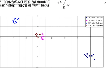
-60 -40 -20 0 20 40 60 80 100
CW Before Calibration CW After Calibration CCW Befor Calibration CCW After Calibration
Figureure 13. Results of UMBmark test in cw and ccw directions before and after calibration for robot
Result of test for correcting wheel base and effective wheel diameter ratio errors are presented. These tests performed with described differential
drive mobile robots. Figures. 13-15 show the results of the uncalibratted runs and calibrated runs in cw and ccw directions for robots.
-100 -80 -60 -40 -20 0 20 40 60
-60 -40 -20 0 20 40 60 80
CW Before Calibration CW After Calibration CCW Befor Calibration CCW After Calibration
Figureure 14. UMBmark test results in two directions before and after calibration for Mobolab
(case II)
-40 -20 0 20 40
-40 -20 0 20 40
CW Before Calibration CW After Calibration CCW Befor Calibration CCW After Calibration
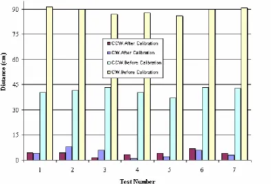
Figures. 16 and 17 show the effect of errors in robot motion in cw and ccw directions. These data obtained from experimental tests and vehicles are shown in average errors. For comparison between robots operations before and after calibration the end position of robots in cw and ccw directions are presented in Figures 18 to 20. The bars in Figureures show the final position of robots that calculated by Eqs. (14) and (15).
After conducting the UMBmark experiments for
minimizing the effect of non systematic errors, suggested to consider the centre of odometry errors in cw and ccw directions. The absolute offsets of two centres of gravity are given by:
(
) (
)
2. . ., . 2
. . ., . .
. .,
.g cw cg cw cg cw
c
x
y
r
=
+
(14)(
) (
)
2. . . ., . 2 . . . ., . .
. . .,
.g ccw cg ccw cg ccw
c
x
y
r
=
+
(15)Figureure 16. UMBmark test path in cw direction for differential drive robots case I, II and III
Figure. 18. End position of Robotest motion in cw and ccw direction before and after calibration
Figureure 20. End position of Sweeper motion in cw and ccw direction before and after calibration
To compare the accuracy of robot before and after calibration, the absolute offset of two centres of gravity is examined and shown in Figureure 21. for each case.
1
Case I
Case II
Case III
51.12
7.10
45.22
6.7
25.67
2.26
0 10 20 30 40 50 60
A
ver
ag
e o
f E
rr
or
s
(c
m
) in
C
C
W D
ir
ec
tio
n
Case I Case II Case III
Before Calibration
After Calibration
Finally, the large value amount
r
c.g.,c.w. and. . . ., .g ccw c
r
as the measure of odometric accuracy for systematic errors is defined as [18]:(
. ., . . . ., . . .)
max,sys
max
r
cg cw;
r
cg ccwE
=
sys
E
max, is calculated and shown in Table 1 for each differential robot.Table1. Accuracy of systematic errors,
E
max,sys. before and after calibration for tested robotsRobot Emax.SysBefore Calibration
Emax.Sys After Calibration
Improvement
Case I 8.5497.15 11
Case II 9.43101.42 10
Case III 6.2333.39 5
7. STATISTIC ANALYSIS OF ROBOT TESTS RESULT
Performance comparison of robots can be achieved with the help of statistical investigation of test results. Normal distribution can be referred for analysing the results. To be specific, the distance between robot final position and the origin, e is
derived using Eqs. (14) and (15). The robot average error e can be obtained as follows:
e
=n
e
∑
(17) where n is the number of trials. Using d as
difference and δ as standard derivation. The normal distribution curve is depicted using Eq. (18).
( )
2 5 . 0 2
1 ⎟⎟⎠
⎞ ⎜ ⎜ ⎝ ⎛ − −
= δ
π
δ
e x
e x
f (18)
The normal distribution curve is delineated in cw and ccw directions using Eq. (18). The normal distribution curve of transitional error for Robotest is illustrated in Figures 22 and 23.
The error distribution curve can be divided into three main regions:
1. The region between minimum and maximum occurred errors in trials.
2. The region defined between the zero error and minimum error.
3.
The region defined as space with error greater than maximum error.Figureure 23. The normal distribution curve of Robotest errors after calibration
75.4
97.64
80.44 98
0 20 40 60 80 100
C.W. Direction C.C.W Direction
Before Calibration
Considering above error distribution, the error occurrence probability in each zone before and after calibration for cw and ccw movements are calculated for all robots and that of Mobolab is demonstrated in Figureure 25. Performance monitoring of robots can be obtained as follows:
BC AC BC e
e
e
e
P
=
−
(19)where
e
BC is maximum of error before calibration, ACe
is maximum of error after calibration andP
e is error decrease percentage.Using Eq. 19 and result of practical tests on robots, their performance in C.W. and C.C.W. directions are investigated as shown in Figureure 26.
From the above Figureure, it is deduced that Robotest performs the others. This conclusion is again justified with precisely reviewing Figureure 21.
Figureure 25. The error occurrence probability in each zone before and after calibration for C.W. and
C.C.W. movements for Mobolab
8. CONCLUSION
Design and kinematics and dynamics modelling result of an omni directional robot and three differential drive robots were presented. To overcome the systematic errors, the Omni-Directional mobile robot was tested and moved in a different path. The systematic errors were determined and corrected. The experimental results are shown the overall odometry accuracy of the robots. With choosing UMBmark method three differential drive robots tested and the systematic errors were modified and reduced by using the method. The absolute measurements of these errors are compared to the position and orientation of the robots as computed according to odometry data. After finding the error sources, robots calibrated and tested again that result of tests presented. Finally, four mobile robots test results analysis with using Normal Distribution. Operation of each robot in difference state for two differential drive robots presented. At the end comparison between robots Performance was presented.
As a new work, the systematic errors can be obtained from some other tests such as UMBmark method. Also it is possible to design an intelligence system for discover, determine and correct the motion error with using Case Base Reasoning or Neural Network.
REFERENCES
1. Borenstein, J., Everett, H.R. and Feng, L., 1997, “Mobile robot positioning: Sensors and techniques”, J. Robot. Syst., vol. 14, pp. 231– 249.
2. Choi, B.J. and Sreenivasan, S.V., 1999, “Gross motion characteristics of articulated mobile robots with pure rolling capability on smooth uneven surfaces”, IEEE Trans. Robot. Automat. vol. 15, pp. 340–343.
3. Hamdy, A. and Badreddin, E., 1992, “Dynamic modelling of a wheeled mobile robot for identification, navigation and control”, in Proc. IMACS Conf. Modeling and Control of Techno. Syst., pp. 119–128.
4. Rajagopalan, R., 1997, “A generic kinematic formulation for wheeled mobile robots”, J.
Robot. Syst., vol. 14, pp. 77–91.
5. Balakrishna, R. and Ghosal, A., 1995, “Modelling of slip for wheeled mobile robots”, IEEE Trans. Robot. Automat., vol. 11, pp. 126– 132.
6. Scheding, S., Dissanayake, G., Nebot, E.M. and Whyte, D.H., 1999, “Experiment in autonomous navigation of an underground mining vehicle”, IEEE Trans. Robot. Automat., vol. 15, pp. 85–95.
7. Watanabe, K., Shiraishi, Y., Tzafestas S., Tang J. and Fukuda, T., 1998, “Feedback control of an omni-directional autonomous platform for mobile service robots”, J. Intell. Robot. Syst., vol. 22, pp. 315–330.
8. Dickerson, S.L. and Lapin, B.D., 1991, “Control of an omni-directional robotic vehicle with mecanum wheels”, in Proc. Nat. Telesystems Conf., vol. 1, pp. 323–328.
9. Meier, R., Fong, T., Thorpe, C., and Baur, C., 1998,”A Sensor Fusion Based User Interface for Vehicle Teleoperation”.
10. Korayem, M.H., Maddahi, Y. and BaniRostam, T., 2004, “Mechanical Design and Modelling of an Omni-directional Mobile Robot“, 12th Annual Mechanical Engineering Conference, Tarbiat Modarres University.
11. Korayem, M.H., Maddahi, Y. and BaniRostam, T., 2004, “Design, Modeling and Experimental Analysis of Wheeled Mobile Robot”, 3rd IFAC Conference.
12. Korayem, M.H. and Basu, A., 2002,”An Educational Mobile Robot-Measurement of Accuracy” The International Journal of Advance Manufacturing Technology, pp. 236-240.
13. Denavit, R.S., Hartenberg, 1955, “A Kinematic Notation for Lower-Pair Mechanisms Based on Matrices”, ASME Journal, pp. 215-221.
14. Borenstein, J., Everett, H.R. and Feng, L., 1996, “Where am I? Sensors and Methods for Mobile Robot Positioning”, Prepared by the University of Michigan for the Oak Ridge National Lab (ORNL) D&D Program.
15. Borenstien, J. and Feng, L., 1995, “UMB mark: A Benchmark Test for Measuring odometry Errors in Mobile Robots”, SPIE conference on Mobile Robots. 16. Borenstein, J. and Feng, L., 1995, “Correction
Robots“, Proceeding of International conference on Intelligent Robots and systems, pp.569-574.
17. Borenstein, J. and Evans, j., “The omniMate Mobile Robot Design, Implementation and Experimental Results.”, Proceedings of IEEE International Conference on Robotics and
Automation, pp.3505-3510.