Deep Models for Arabic Dialect Identification on Benchmarked Data

Proceedings of the Fifth Workshop on NLP for Similar Languages, Varieties and Dialects, pages 263–274 263

Deep Models for Arabic Dialect Identification on Benchmarked Data

Mohamed Elaraby Muhammad Abdul-Mageed

Natural Language Processing Lab University of British Columbia

mohamed.elaraby@alumni.ubc.ca,muhammad.mageeed@ubc.ca

Abstract

The Arabic Online Commentary (AOC) (Zaidan and Callison-Burch, 2011) is a large-scale repos-itory of Arabic dialects with manual labels for4varieties of the language. Existing dialect iden-tification models exploiting the dataset pre-date the recent boost deep learning brought to NLP and hence the data are not benchmarked for use with deep learning, nor is it clear how much neural networks can help tease the categories in the data apart. We treat these two limitations: We (1) benchmark the data, and (2) empirically test6 different deep learning methods on the task, comparing peformance to several classical machine learning models under different condi-tions (i.e., both binary and multi-way classification). Our experimental results show that variants of (attention-based) bidirectional recurrent neural networks achieve best accuracy (acc) on the task, significantly outperforming all competitive baselines. On blind test data, our models reach

87.65%acc on the binary task (MSA vs. dialects),87.4%acc on the 3-way dialect task (Egyptian vs. Gulf vs. Levantine), and82.45%acc on the 4-way variants task (MSA vs. Egyptian vs. Gulf vs. Levantine). We release our benchmark for future work on the dataset.

1 Introduction

Dialect identification is a special type of language identification where the goal is to distinguish closely related languages. Explosion of communication technologies and the accompanying pervasive use of social media strongly motivates need for technologies like language, and dialect, identification. These technologies are useful for applications ranging from monitoring health and well-being (Yepes et al., 2015; Nguyen et al., 2016; Nguyen et al., 2017; Abdul-Mageed et al., 2017), to real-time disaster op-eration management (Sakaki et al., 2010; Palen and Hughes, 2018), and analysis of human mobility (Hawelka et al., 2014; Jurdak et al., 2015; Louail et al., 2014). Language identification is also an en-abling technology that can help automatically filter foreign text in some tasks (Lui and Baldwin, 2012), acquire multilingual data (e.g., from the web) (Abney and Bird, 2010), including to enhance tasks like machine translation (Ling et al., 2013).

Arabic. In this paper our focus is onArabic, a term that refers to a wide collection of varieties. These varieties are the result of the interweave between the native languages of the Middle East and North Africa and Arabic itself. Modern Standard Arabic (MSA), the modern variety of the language used in pan-Arab news outlets like AlJazeera and in educational circles in the Arab world, differs phonetically, phonologically, lexically, and syntactically from the varieties spoken in everyday communication by native speakers of the language (Diab et al., 2010; Habash, 2010; Abdul-Mageed, 2015; Abdul-Mageed, 2017). These ‘everyday’ varieties constitute the dialects of Arabic. Examples of these are Egyptian (EGY), Gulf (GLF), Levantine (LEV), and Moroccan (MOR). In addition to MSA and dialects, Classical Arabic also exists and is the variety of historical literary texts and religious discourse.

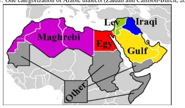
Arabic Dialects. Language varieties, including those of Arabic, can be categorized based on shared linguistic features. For Arabic, one classical categorization is based on geographical locations. For example, in addition to MSA, Habash et al. (2012), provides 5 main categories, as shown in Figure 1. This same classification is also common in the literature, and includes:

• Egyptian: The variety spoken in Egypt, which is widely spread due to the historical impact of Egyptian media

• Gulf:A variety spoken primarily in Saudi Arabia, UAE, Kuwait and Qatar

• Iraqi:The variety spoken by the people of Iraq

• Levantine: The variety spoken primarily by the Levant (i.e., people of Syria, Lebanon, and Pales-tine)

• Maghrebi:The variety spoken by people of North Africa, excluding Egypt

Figure 1: One categorization of Arabic dialects (Zaidan and Callison-Burch, 2011)

Arabic dialectal data. For a long time, Arabic dialects remained mostly spoken. Dialects started to find their way in written form with the spread of social media, thus affording an opportunity for researchers to use these data for NLP. This motivated Zaidan and Callison-Burch (2014) to create a large-scale repository of Arabic texts, the Arabic Online Commentary (AOC). The resource is composed of∼3M MSA and dialectal comments on a number of Arabic news sites. A portion of the data (>108K comments) is manually annotated via crowdsourcing. The dataset was exploited for dialect identification in Zaidan and Callison-Burch (2014) and later in Cotterell and Callison-Burch (2014). These works, however, pre-date the current boom in NLP where deep neural networks enable better learning (given sufficiently large training data). Cotterell and Callison-Burch (2014) usen-fold cross validation in their work, thus making it costly to adopt the same data split procedure to develop deep learning models. This is the case since deep models can take long times to train and optimize. For this reason, it is desirable to benchmark the AOC dataset for deep learning research. This motivates our work. We also ask the empirical question: To what extent can we tease apart the Arabic varieties in AOC using neural networks. Especially given (a) the morphological richness of Arabic and (b) the inter-relatedness (e.g., lexical overlap) between Arabic varieties, it is not clear how accurately these varieties can be automatically categorized (using deep learning methods). To answer these important questions, we investigate the utility of several traditional machine learning classifiers and6different deep learning models on the task. Our deep models are based on both recurrent neural networks and convolutional neural networks, as well as combinations (and variations) of these.

Overall, we offer the following contributions: (1) We benchmark the AOC dataset, especially for deep learning work, (2) we perform extensive experiments based on deep neural networks for identifying the

Variety Example

MSA

(1)_{Õ»Ygð àðQ‚ B Õ æ K@ , A JJ.j JÓ AK éÒêÖÏ@ @ðY ƒ} Go, go, our team; you’ve our passionate support. (2)_{Q k@ I}

. .ƒ ø@ úæk Bð éʪ ®Ë@ è Yë PQ.K Éêm.Ì'@ C ¯ ÐC¾Ë@ á« H Qj.« Y®Ë ék@Qå”.

Frankly, I’m speechless. Neither ignorance nor any other reason justify this action.

EGY

(3)_{Õ»Q ¢ ú}

¯ áÓQm.× @ñ KA¿ð éÓ PB@ @ðQm.¯ A JJKA ’¯ð A JÓC«@ à@ @ñËñ ®JK.

You say our media and satellite channels initiated the crisis and were criminals in your review. (3)_{ñm.Ì'@ ú¯ ­ÊK QÒ®Ë@ ¬Q« ñËÒ ‚ÖÏ@ ú}

¯ ,14 QÔ ¯ Bð ú

«A J“ QÔ ¯

Either its a satellite or a full moon [playful for “beautiful female”], it will never rotate in its orbit correctly.

GLF

(5)_{é®JJ.¢ ú}

¯ ÑëAƒ áÓð P@Q

®Ë@ @Yë hQ¯@ áÓ úΫ éJ¯AªË@ ù ¢ªK

Healthy be the one who proposed this decision, and those who contributed in applying it. (6)_Zú

æ… àñÊ ªJ ‚ àñ ªJ.K Bð ÑîD ®ºK Bð Zúæ… ÑîD“QK AÓ €A JË@ ‘ªK. A KY J«

Nothing would please nor be enough for some of these people; they don’t even want to put any efforts.

LEV

(7)_{AîD¯ @ñÊ®ºJK. øñ} k@ð ø _{ñK.@ð úÍAK. úΫ Bð úGPAJƒ iʒ. B} àAÒ» A K@ð And I also won’t repair my car, nor do I care. My brother and dad will take care of it. (8)éªÓAm.Ì'@ I.Ê¢Ë ÑîEA«A ƒ@ I..‚. éʾ ‚Ó àñJÊÓ Q’ hP I KA¿ð ék.PYÊêË PñÓB@ ɓñK Èñ®ªÓ ñÓ àB

Because it isn’t reasonable for things to get to that bad. There is a million problems college students have because of their rumors.

Table 1: Example comments from the4varieties in the AOC dataset

where we describe our experimental set up, Section 6 provides our experimentation results. Section 7 is a visualization-based analysis of our results. Section 8 is where we conclude our work and overview future directions.

2 Related work

Work on Arabic dialect identification has focused on both spoken (Ali et al., 2015; Belinkov and Glass, 2016; Najafian et al., 2018; Shon et al., 2018; Shon et al., 2017; Najafian et al., 2018) and written form (Elfardy and Diab, 2013; Zaidan and Callison-Burch, 2014; Cotterell and Callison-Burch, 2014; Darwish et al., 2014; Abdul-Mageed et al., 2018). Early works have focused on distinguishing between MSA and EGY. For example, Elfardy and Diab (2013) propose a supervised method for sentence-level MSA-EGY categorization, exploiting a subset of the AOC dataset (12,160MSA sentences and11,274

of user commentaries on Egyptian news articles). The authors study the effect of pre-processing on classifier performance, which they find to be useful under certain conditions. Elfardy and Diab (2013) report 85.5% accuracy using 10-fold cross-validation with an SVM classifier, compared to the 80.9%

accuracy reported by Zaidan and Callison-Burch (2011). Similarly, Tillmann et al. (2014) exploit the same portion of the AOC data Elfardy and Diab (2013) worked on, to build an MSA-EGY classifier. The authors report an improvement of1.3%over results acquired by Zaidan and Callison-Burch (2014) using a linear classifier utilizing an expanded feature set. Their features include n-grams defined via part of speech tags and lexical features based on the AIDA toolkit (Elfardy et al., 2014). The work of Darwish et al. (2014) is also similar to these works in that it also focuses on the binary MSA-EGY classification task, but the authors exploit Twitter data. More specifically, Darwish et al. (2014) collected a dataset of 880K tweets on which they train their system, while testing on 700 tweets they labeled for the task. The authors explore a range of lexical and morphological features and report a10%absolute gain over models trained with n-grams only. Our work is similar to these works in that we exploit the AOC dataset and develop MSA-EGY, binary classifiers. However, we model the task at more fine-grained levels as well (i.e., 3-way and 4-way classification).

nor benchmark the task on AOC. Their results are not directly comparable to our work for these reasons. Finally, our work has some similarity to general works on language detection (Jurgens et al., 2017; Jauhiainen et al., 2017; Kocmi and Bojar, 2017; Jauhiainen et al., 2018) and geographical location (Rahimi et al., 2018; Mahmud et al., 2014; Rahimi et al., 2017).

3 Dataset: Arabic Online Commentary (AOC)

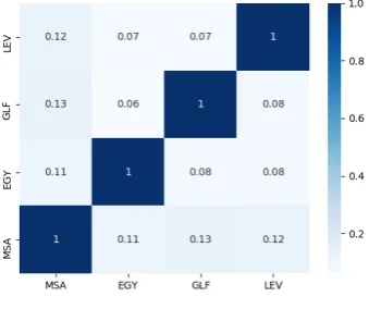
As we mentioned earlier, our work is based on the AOC dataset. AOC is composed of 3M MSA and dialectal comments, of which108,173comments are labeled via crowdsourcing. For our experiments, we randomly shuffle the dataset and split it into80%training (Train), 10% validation (Dev), and 10% test (Test). Table 2 shows the distribution of the data across the different splits. We were interested in identifying how the4 varieties relate to one another in terms of their shared vocabulary, and so we performed an analysis on the training split (Train) as shown in the heat map in Figure 2. The Figure presents the percentages of shared vocabulary between the different varieties after normalizing for the number of data points in each class. As the Figure shows, both the GLF and LEV dialects are lexically closer to (i.e., share more vocabulary with) MSA than EGY is (does). This finding is aligned with the intuition of native speakers of Arabic that EGY diverges more from MSA than the GLF and LEV varieties. This empirical finding lends some credibility to this intuition.

Table 2: Distribution of classes in our AOCTrainsplit

Variety MSA EGY GLF LEV ALL

Train 50,845 10,022 16,593 9,081 86,541

Dev 6,357 1,253 2,075 1,136 10,821

Test 6,353 1,252 2,073 1,133 10,812

Figure 2: Heat map for shared vocabulary between different data variants

4 Models

4.1 Traditional models

Traditional models refer to models based on feature engineering methods with linear and probabilistic classifiers. In our experiments, we use (1) logistic regression, (2) multinomial Naive Bayes, and (3) support vector machines (SVM) classifiers.

4.2 Deep Learning Models

BiLSTM with attention. While there are other variations of how some of these models learn (Vaswani et al., 2017), we believe these models with the variations we exploit form a strong basis for our bench-marking objective. In all our models, we use pre-trained word vectors based on word2vec to initialize the networks. We then fine-tune weights during learning.

Word-based Convolutional Neural Network (CNN):This model is conceptually similar to the one described in Kim (2014), and has the following architecture:

• Input layer: an input layer to map word sequencewinto a sequence vector xwherexw is a real-valued vector (xw ∈Rdemb_{, withdemb= 300in all our models) initialized from external embedding} model and tuned during training. The embedding layer is followed by a dropout rate of 0.5 for regularization (in this case to prevent co-adaptation between hidden units).

• Convolution layer: Two 1-D convolution operations are applied in parallel to the input layer to map input sequence x into a hidden sequence h. A filter k ∈ _Rwdemb _{is applied to a window} of concatenated word embedding of size w to produce a new featureci . Where ci ∈ R , ci = kxi:i+w−1+b, b is the biasb ∈ R, andxi:i+w−1 is a concatenation ofxi, ...xi+w1. The filter

sizes used are 3 and 8 and the number of filters used is 10. After each convolution operation a non-linear activation of type Rectifier Linear Unit (ReLU) (Nair and Hinton, 2010) is applied. Finally different convolution outputs (the two convolutional maps in our case) are concatenated into a sequencec ∈_Rn−h+1_{(wherenis the number of filters andhis the dimensionality of the hidden}

sequence) and passed to a pooling layer.

• Maxpooling:Temporal max-pooling, which is the 1-D version of pooling, is applied over the con-catenated output of the multiple convolutionsc, as mentioned above. The sequencecis converted into a single hidden vectorc0by taking the maximum values of extracted feature mapc0 =max{c}. The size ofc0isΣiniwiwhereniis the number of filters andwi the width of these filters.

• Dense layer: A100dimension fully-connected layer with a ReLU non-linear activation is added to map vectorc0 into a final vectorc00. For regularization, we employ a dropout rate of0.8and an l2-norm.

• Softmax layer: Finally, the hidden units c00 is converted into probability distribution over l via softmax function, wherelis the number of classes.

Long-Short Term Memory (LSTM): In our experiments, we use different variations of recurrent neural networks. The first one is LSTM (Hochreiter and Schmidhuber, 1997). We use a word-based LSTM, with the following architecture:

• Input layer:The input layer is exactly the same as the one described in the CNN model above.

• LSTM layer: We use a vanilla LSTM architecture consisting of100dimensions hidden units. The LSTM is designed to capture long-term dependencies via augmenting a standard RNN with a mem-ory stateCt, withCt ∈Rat time stept. The LSTM takes in a previous stateht−1and inputxt, to calculate the hidden statehtas follows:

it=σ(Wi.[ht−1, xt] +bi)

ft=σ(Wf.[ht−1, xt] +bf) ˜

Ct=tanh(WC.[ht−1, xt] +bC)

Ct=ftCt−1+itC˜

ot=σ(Wo[ht−1, xt] +bo)

ht=ottanh(Ct)

(1)

vector with candidates that could be added to the state. We use the same regularization as we apply on the dense layer in the CNN model mentioned above.

• Softmax layer:Similar to that of the CNN above as well.

Convolution LSTM (CLSTM):This model is described in Zhou et al. (2015). The model archi-tecture is similar to the CNN described earlier, but the fully-connected (dense) layer is replaced by an LSTM layer. The intuition behind the CLSTM is to use the CNN layer as a feature extractor, and directly feed the convolution output to the LSTM layer (which can capture long-term dependencies).

Bidirectional LSTM (BiLSTM):One limitation of conventional RNNs is that they are able to make predictions based on previously seen content only. Another variant of RNNs that addresses this problem is Bidirectional RNNs (BRNNs), which process the data in both directions in two separate hidden layers. These two hidden layers are then fed forward to the same output layer. BRNNs compute three sequences; a forward hidden sequence−→h, a backward hidden sequence←−h, and the output sequencey. The model transition equations are as below:

− →

h =H(W_x−→

hxt+W−→h−→h

− →

ht+1+b−→_h) ←−

h =H(W_x←−

hxt+W←−h←h−

←−

ht+1+b←−_h)

yt=W−→_{h y}

− →

ht+W←−_{h y}

←−

ht+by

(2)

WhereHcan be any activation function. Combining BRNN and LSTM gives the BiLSTM model. In our experiments we use a100hidden units dimension to ensure a fair comparison with LSTM’s results. We apply the same regularization techniques applied for the LSTM layer described above.

Bidirectional Gated Recurrent Units (BiGRU):Gated Recurrent Unit (GRU) (Chung et al., 2014) is a variant of LSTMs that combines theforgetandinputgates into a single update gateztby primarily merging thecellstate andhiddenstate. This results in a simpler model composed of anupdatestatezt, aresetstatert, and a new simplerhiddenstateht. The model transition equations are as follows:

zt=σ(Wz.[ht−1, xt])

rt=σ(Wr.[ht−1, xt])

˜

ht=tanh(W.[rt∗ht−1, xt])

ht= (1−zt)∗ht−1+zt∗ht˜

(3)

The Bidirectional GRU (BiGRUs) can be obtained by combining two GRUs, each looking at a different direction similar to the case of BiLSTMs above. We employ the same regularization techniques applied to the LSTM and BiLSTM networks.

Attention-based BiLSTM

Recently, using an attention mechanism with a neural networks has resulted in notable success in a wide range of NLP tasks, such as machine translation, speech recognition, and image captioning (Bah-danau et al., 2014; Xu et al., 2015; Chorowski et al., 2015). In this section, we describe an attention mechanism that we employ in one of our models (BiLSTM) that turned out to perform well without attention, hoping the mechanism will further improve model performance. We use a simple implementa-tion inspired by Zhou et al. (2016) where attenimplementa-tion is applied to the output vector of the LSTM layer. If His a matrix consisting of output vectors[h1, h2, ..hT](whereTis the sentence length), we can compute the attention vectorαof the sequence as follows:

et=tanh(ht)

αt=

exp(et)

ΣT

i=1exp(ei)

Finally, the representation vector for input textvis computed by a weighted summation over all the time steps, using obtained attention scores as weights.

v= ΣT_i=1αihi (5)

The vectorvis an encoded representation of the whole input text. This representation is passed to the sof tmaxlayer for classification.

5 Experiments

We perform 3 different classification tasks: (A) binary classification, where we tease apart the MSA and the dialectal data, (B) 3-way dialects, where we attempt to distinguish between EGY, GLF, and LEV; and (C)4-way variants(i.e., MSA vs. EGY vs. GLF vs. LEV). Since our goal in this work is to explore how several popular traditional settings and deep learning model architectures fare on the dialect identification task, we use classifiers with pre-defined hyper-parameters inspired by previous works as described in Section 4. As we mention in Section 3, we split the data into 80%Train, 10%Dev, and 10% Test. While we train onTrainand report results on both theDevandTestsets in the current work, our goal is to invest on hyper-parameter tuning based on the development set in the future. Benchmarking the data is thus helpful as it facilitates comparisons in future works. 1

5.1 Pre-processing

We process our data the same way across all our traditional and deep learning experiments, as follows:

• Tokenization and normalization: We tokenize our data based on white space, excluding all non-unicode characters. We then normalizeAlif maksuratoYa, reduce allhamzated Alif to plain Alif, and remove all non-Arabic characters/words (e.g., “very”, “50$”).

• Input sequence quantization:In our experiments, we fix the vocabulary at the most frequent 50K words. The input tokens are then converted into indices ranging from 1 to 50K based on our look-up vocabulary.

• Padding: For the deep learning classifiers, all input sequences are truncated to arbitrary maximum sequence length of 30 words per comment. Comments of length<30 are zero-padded. This number can be tuned in future work.

5.2 Traditional Classifier Experiments

We have two settings for the traditional classifiers: (1) presence vs. absence (0 vs. 1) vectors based on combinations of unigrams, bigrams, and trigrams; and (2) term-frequency inverse-document-frequency (TF-IDF) vectors based on combinations of unigrams, bigrams, and trigrams (Sparck Jones, 1972). We use scikit-learn’s (Pedregosa et al., 2011) implementation of these classifiers.

5.3 Deep Learning Experiments

All our deep models are trained for 10 epochs using the RMSprop optimizer. The model’s weightsW are initialized from a normal distributionW ∼ N with a small standard deviation ofσ = 0.05. Our models are trained using the Keras (Chollet and others, 2015) library with a Tensorflow (Abadi et al., 2016) backend. We train each of our 6 deep learning classifiers across 3 different settings pertaining the way we initialize the embeddings for the input layer in each network. The three embedding settings are:

1. Random embeddings:Where we initialize the input layer randomly.

2. AOC-based embeddings: We make use of the∼ 3M unlabeled comments in AOC by training a “continuous bag of words” (CBOW) (Mikolov et al., 2013) model exploiting them. We adopt the settings in Abdul-Mageed et al. (2018) for training our model to acquire 300 dimensional word vectors.

Binary Three-way Four-way

Method Dev Test Dev Test Dev Test

Traditional Classifiers

Baseline (majority class inTrain) 58.75 58.75 58.75 58.75 46.49 46.49 Logistic Regression (1+2+3 grams) 84.18 83.71 86.91 85.75 75.75 78.24 Naive Bayes (1+2+3 grams) 84.97 84.53 87.51 87.81 80.15 77.75

SVM (1+2+3 grams) 82.79 82.41 85.51 84.27 74.5 75.82

Logistic Regression (1+2+3 grams TF-IDF) 83.96 83.24 86.71 85.51 75.81 78.24 Naive Bayes (1+2+3 grams TF-IDF) 83.52 82.91 86.61 86.87 73.21 75.81 SVM (1+2+3 grams TF-IDF) 84.07 83.61 86.76 85.93 76.65 78.61

Deep Learning - Random Embeddings

CNN (Kim, 2014) 85.69 85.16 81.63 81.11 66.34 68.86

CLSTM (Zhou et al., 2015) 84.73 84.17 78.91 78.32 64.58 65.25

LSTM 85.41 85.28 78.61 78.51 70.21 68.71

BiLSTM 84.11 83.77 85.82 84.99 75.94 77.55

BiGRU 82.81 82.77 84.88 84.45 74.56 76.51

Attention-BiLSTM 85.5 85.23 86.12 85.93 79.97 80.21

Deep Learning - AOC Embeddings

CNN (Kim, 2014) 85.02 84.51 76.81 76.53 64.23 64.17

CLSTM (Zhou et al., 2015) 85.17 84.73 76.81 75.71 64.61 63.89

LSTM 85.04 84.07 83.89 82.67 70.01 68.91

BiLSTM 85.33 84.88 86.21 86.01 76.12 78.35

BiGRU 85.39 85.27 86.92 86.57 79.61 80.11

Attention-BiLSTM 85.77 85.71 87.01 86.93 80.25 81.12

Deep Learning - Twitter-City Embeddings (Abdul-Mageed et al., 2018)

CNN (Kim, 2014) 86.68 86.26 85.51 85.36 74.13 75.61

CLSTM (Zhou et al., 2015) 86.61 86.28 82.77 82.56 79.41 77.51

LSTM 85.52 85.07 84.41 84.61 75.21 78.53

BiLSTM 87.16 86.99 87.31 87.11 82.81 81.93

BiGRU 87.65 87.23 87.11 86.18 83.25 82.21

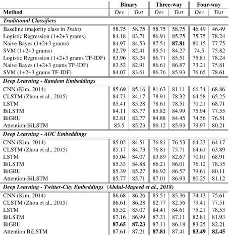
Attention BiLSTM 87.61 87.21 87.81 87.41 83.49 82.45

Table 3: Experimental results, in accuracy, on ourDevandTestAOC splits

3. Twitter-City embeddings: This is based on the CBOW word2vec model released by Abdul-Mageed et al. (2018). The authors train their models on a1₄ billion tweets dataset collected from 29 different cities from 10 Arab countries. The authors use a window of size 5 words, minimal word frequency set at 100 words, and 300 dimensional word vectors to train this model.

6 Results

Table 3 shows our results in accuracy across the three classification tasks (i.e., binary, 3-way, and 4-way), as described in Section 5. Our baseline in each task is the majority class in the respectiveTrainset. As Table 6 shows, among traditional models, the Naive Bayes classifier achieves the best performance across all three tasks both onDevandTestdata. As a sole exception, SVMs outperforms Naive Bayes on theTestset for the 4-way classification task. As best accuracy, traditional classifiers yield84.53(binary),

87.81(3-way), and78.61(4-way) on theTestsplits.

with the AOC embeddings. We also observe that AOC embeddings are better than random initialization. Forbinary classification, as Table 6 shows, BiGRU obtains the best accuracy on bothDev(87.65) and Test(87.23), with attention-BiLSTM performing quite closely. For the3-way classificationtask (dialect only classifier), while attention-BiLSTM obtains the best result on theDev(87.81), it is slightly outper-formed by the Naive Bayes classifier onTest(also87.81). For4-way classification, attention-BiLSTM obtained best accuracy on bothDev(83.49) andTest(82.42).

Aligned with knowledge about deep models, we note the positive effect of larger training data on classification. For example, when we reduce the size ofTrainby excluding the MSA comments (58%of the manually annotated data), traditional classifiers outperform most of the deep learning classifiers on 3-way classification. Similarly, results drop when we thinly spread the data across the 4 categories for 4-way classification.

7 Analysis

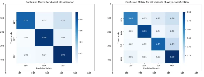
Figure 3 is a visualization of classification errors acquired with attention-BiLSTM results (best accuracy in the multi-class tasks). Theleft-side (3-way/dialects)matrix shows how LEV is confused20%of the time with GLF, directly reflecting the closer lexical distance between the two varieties compared to the distance of either of them to EGY. Theright-side (4-way)matrix shows that23%of the GLF errors are confused with MSA, followed by LEV errors (confused with MSA20%of the time). This is a result of the higher lexical overlap between the two dialects and MSA, as we described in our observations around Figure 2. As Table 2 shows, MSA also dominatesTrainand hence these confusions with MSA are expected.

Figure 3: Analysis of Attention-BiLSTM results.Left:Confusion matrix for3-waypredictions.Right: Confusion matrix for4-wayclassification.

8 Conclusion

We benchmarked the AOC dataset, a popular dataset of Arabic online comments, for deep learning work focused at dialect identification. We also developed12different classifiers (6traditional and6based on deep learning) to offer strong baselines for the task. Results show attention-based BiLSTMs to work well on this task, especially when initialized using a large dialect specific word embeddings model. In the future, we plan to exploit sub-word and further tune hyper-parameters of our models.

9 Acknowledgement

References

Mart´ın Abadi, Paul Barham, Jianmin Chen, Zhifeng Chen, Andy Davis, Jeffrey Dean, Matthieu Devin, Sanjay Ghemawat, Geoffrey Irving, Michael Isard, et al. 2016. Tensorflow: A system for large-scale machine learning. InOSDI, volume 16, pages 265–283.

Muhammad Abdul-Mageed, Anneke Buffone, Hao Peng, Johannes C Eichstaedt, and Lyle H Ungar. 2017. Rec-ognizing pathogenic empathy in social media. InICWSM, pages 448–451.

Muhammad Abdul-Mageed, Hassan Alhuzali, and Mohamed Elaraby. 2018. You tweet what you speak: A city-level dataset of arabic dialects. InLREC, pages 3653–3659.

Muhammad Abdul-Mageed. 2015. Subjectivity and sentiment analysis of Arabic as a morophologically-rich language. Ph.D. thesis, Indiana University.

Muhammad Abdul-Mageed. 2017. Modeling arabic subjectivity and sentiment in lexical space. Information Processing & Management.

Steven Abney and Steven Bird. 2010. The human language project: building a universal corpus of the world’s languages. InProceedings of the 48th annual meeting of the association for computational linguistics, pages 88–97. Association for Computational Linguistics.

Ahmed Ali, Najim Dehak, Patrick Cardinal, Sameer Khurana, Sree Harsha Yella, James Glass, Peter Bell, and Steve Renals. 2015. Automatic dialect detection in arabic broadcast speech. arXiv preprint arXiv:1509.06928.

Dzmitry Bahdanau, Kyunghyun Cho, and Yoshua Bengio. 2014. Neural machine translation by jointly learning to align and translate. arXiv preprint arXiv:1409.0473.

Yonatan Belinkov and James Glass. 2016. A character-level convolutional neural network for distinguishing similar languages and dialects. arXiv preprint arXiv:1609.07568.

Franc¸ois Chollet et al. 2015. Keras.

Jan K Chorowski, Dzmitry Bahdanau, Dmitriy Serdyuk, Kyunghyun Cho, and Yoshua Bengio. 2015. Attention-based models for speech recognition. InAdvances in neural information processing systems, pages 577–585.

Junyoung Chung, Caglar Gulcehre, KyungHyun Cho, and Yoshua Bengio. 2014. Empirical evaluation of gated recurrent neural networks on sequence modeling. arXiv preprint arXiv:1412.3555.

Ryan Cotterell and Chris Callison-Burch. 2014. A multi-dialect, multi-genre corpus of informal written arabic. In

LREC, pages 241–245.

Kareem Darwish, Hassan Sajjad, and Hamdy Mubarak. 2014. Verifiably effective arabic dialect identification. In

Proceedings of the 2014 Conference on Empirical Methods in Natural Language Processing (EMNLP), pages

1465–1468.

Mona Diab, Nizar Habash, Owen Rambow, Mohamed Altantawy, and Yassine Benajiba. 2010. Colaba: Arabic dialect annotation and processing. InLrec workshop on semitic language processing, pages 66–74.

Heba Elfardy and Mona Diab. 2013. Sentence level dialect identification in arabic. InProceedings of the 51st

Annual Meeting of the Association for Computational Linguistics (Volume 2: Short Papers), volume 2, pages

456–461.

Heba Elfardy, Mohamed Al-Badrashiny, and Mona Diab. 2014. Aida: Identifying code switching in informal arabic text. In Proceedings of The First Workshop on Computational Approaches to Code Switching, pages 94–101.

Nizar Habash, Mona T Diab, and Owen Rambow. 2012. Conventional orthography for dialectal arabic. InLREC, pages 711–718.

Nizar Y Habash. 2010. Introduction to arabic natural language processing. Synthesis Lectures on Human Lan-guage Technologies, 3(1):1–187.

Bartosz Hawelka, Izabela Sitko, Euro Beinat, Stanislav Sobolevsky, Pavlos Kazakopoulos, and Carlo Ratti. 2014. Geo-located twitter as proxy for global mobility patterns. Cartography and Geographic Information Science, 41(3):260–271.

Fei Huang. 2015. Improved arabic dialect classification with social media data. InProceedings of the 2015

Conference on Empirical Methods in Natural Language Processing, pages 2118–2126.

Tommi Jauhiainen, Krister Lind´en, and Heidi Jauhiainen. 2017. Evaluation of language identification methods using 285 languages. InProceedings of the 21st Nordic Conference on Computational Linguistics, pages 183– 191.

Tommi Jauhiainen, Marco Lui, Marcos Zampieri, Timothy Baldwin, and Krister Lind´en. 2018. Automatic lan-guage identification in texts: A survey. arXiv preprint arXiv:1804.08186.

Raja Jurdak, Kun Zhao, Jiajun Liu, Maurice AbouJaoude, Mark Cameron, and David Newth. 2015. Understanding human mobility from twitter.PloS one, 10(7):e0131469.

David Jurgens, Yulia Tsvetkov, and Dan Jurafsky. 2017. Incorporating dialectal variability for socially equi-table language identification. InProceedings of the 55th Annual Meeting of the Association for Computational Linguistics (Volume 2: Short Papers), volume 2, pages 51–57.

Yoon Kim. 2014. Convolutional neural networks for sentence classification.arXiv preprint arXiv:1408.5882.

Tom Kocmi and Ondˇrej Bojar. 2017. Lanidenn: Multilingual language identification on character window. arXiv preprint arXiv:1701.03338.

Wang Ling, Guang Xiang, Chris Dyer, Alan Black, and Isabel Trancoso. 2013. Microblogs as parallel corpora.

InProceedings of the 51st Annual Meeting of the Association for Computational Linguistics (Volume 1: Long

Papers), volume 1, pages 176–186.

Thomas Louail, Maxime Lenormand, Oliva G Cantu Ros, Miguel Picornell, Ricardo Herranz, Enrique Frias-Martinez, Jos´e J Ramasco, and Marc Barthelemy. 2014. From mobile phone data to the spatial structure of cities. Scientific reports, 4:5276.

Marco Lui and Timothy Baldwin. 2012. langid. py: An off-the-shelf language identification tool. InProceedings of the ACL 2012 system demonstrations, pages 25–30. Association for Computational Linguistics.

Jalal Mahmud, Jeffrey Nichols, and Clemens Drews. 2014. Home location identification of twitter users. ACM Transactions on Intelligent Systems and Technology (TIST), 5(3):47.

Tomas Mikolov, Kai Chen, Greg Corrado, and Jeffrey Dean. 2013. Efficient estimation of word representations in vector space. arXiv preprint arXiv:1301.3781.

Vinod Nair and Geoffrey E Hinton. 2010. Rectified linear units improve restricted boltzmann machines. In

Proceedings of the 27th international conference on machine learning (ICML-10), pages 807–814.

Maryam Najafian, Sameer Khurana, Suwon Shon, Ahmed Ali, and James Glass. 2018. Exploiting convolutional neural networks for phonotactic based dialect identification. ICASSP.

Quynh C Nguyen, Dapeng Li, Hsien-Wen Meng, Suraj Kath, Elaine Nsoesie, Feifei Li, and Ming Wen. 2016. Building a national neighborhood dataset from geotagged twitter data for indicators of happiness, diet, and physical activity.JMIR public health and surveillance, 2(2).

Quynh C Nguyen, Kimberly D Brunisholz, Weijun Yu, Matt McCullough, Heidi A Hanson, Michelle L Litchman, Feifei Li, Yuan Wan, James A VanDerslice, Ming Wen, et al. 2017. Twitter-derived neighborhood characteris-tics associated with obesity and diabetes. Scientific reports, 7(1):16425.

Leysia Palen and Amanda L Hughes. 2018. Social media in disaster communication. InHandbook of Disaster Research, pages 497–518. Springer.

Fabian Pedregosa, Ga¨el Varoquaux, Alexandre Gramfort, Vincent Michel, Bertrand Thirion, Olivier Grisel, Math-ieu Blondel, Peter Prettenhofer, Ron Weiss, Vincent Dubourg, et al. 2011. Scikit-learn: Machine learning in python. Journal of machine learning research, 12(Oct):2825–2830.

Afshin Rahimi, Trevor Cohn, and Timothy Baldwin. 2017. A neural model for user geolocation and lexical dialectology.arXiv preprint arXiv:1704.04008.

Takeshi Sakaki, Makoto Okazaki, and Yutaka Matsuo. 2010. Earthquake shakes twitter users: real-time event detection by social sensors. In Proceedings of the 19th international conference on World wide web, pages 851–860. ACM.

Suwon Shon, Ahmed Ali, and James Glass. 2017. Mit-qcri arabic dialect identification system for the 2017 multi-genre broadcast challenge. arXiv preprint arXiv:1709.00387.

Suwon Shon, Ahmed Ali, and James Glass. 2018. Convolutional neural networks and language embeddings for end-to-end dialect recognition. arXiv preprint arXiv:1803.04567.

Karen Sparck Jones. 1972. A statistical interpretation of term specificity and its application in retrieval. Journal of documentation, 28(1):11–21.

Christoph Tillmann, Saab Mansour, and Yaser Al-Onaizan. 2014. Improved sentence-level arabic dialect clas-sification. InProceedings of the First Workshop on Applying NLP Tools to Similar Languages, Varieties and Dialects, pages 110–119.

Ashish Vaswani, Noam Shazeer, Niki Parmar, Jakob Uszkoreit, Llion Jones, Aidan N Gomez, ukasz Kaiser, and Illia Polosukhin. 2017. Attention is all you need. InAdvances in Neural Information Processing Systems, pages 6000–6010.

Yan Xu, Lili Mou, Ge Li, Yunchuan Chen, Hao Peng, and Zhi Jin. 2015. Classifying relations via long short term memory networks along shortest dependency paths. InProceedings of the 2015 Conference on Empirical

Methods in Natural Language Processing, pages 1785–1794.

Antonio Jimeno Yepes, Andrew MacKinlay, and Bo Han. 2015. Investigating public health surveillance using twitter. Proceedings of BioNLP 15, pages 164–170.

Omar F Zaidan and Chris Callison-Burch. 2011. The arabic online commentary dataset: an annotated dataset of informal arabic with high dialectal content. InProceedings of the 49th Annual Meeting of the Association for

Computational Linguistics: Human Language Technologies: short papers-Volume 2, pages 37–41. Association

for Computational Linguistics.

Omar F Zaidan and Chris Callison-Burch. 2014. Arabic dialect identification. Computational Linguistics, 40(1):171–202.

Chunting Zhou, Chonglin Sun, Zhiyuan Liu, and Francis Lau. 2015. A c-lstm neural network for text classifica-tion. arXiv preprint arXiv:1511.08630.