Principal Component Analysis of Image Gradient Orientations for Face
Recognition
Georgios Tzimiropoulos
†, Stefanos Zafeiriou
†and Maja Pantic
†,∗†
Department of Computing, Imperial College London
180 Queen’s Gate, London SW7 2AZ, UK.
∗
EEMCS, University of Twente, 5 Drienerlolaan,
7522 NB Enschede, The Netherlands.
{
gt204, s.zafeiriou,m.pantic
}
@imperial.ac.uk
Abstract— We introduce the notion of Principal Component Analysis (PCA) of image gradient orientations. As image data is typically noisy, but noise is substantially different from Gaussian, traditional PCA of pixel intensities very often fails to estimate reliably the low-dimensional subspace of a given data population. We show that replacing intensities with gradient orientations and the ℓ2 norm with a cosine-based distance measure offers, to some extend, a remedy to this problem. Our scheme requires the eigen-decomposition of a covariance matrix and is as computationally efficient as standard ℓ2 intensity-based PCA. We demonstrate some of its favorable properties for the application of face recognition.
NOTATION S,{.} set
ℜ set of reals
C set of complex numbers x scalar or complex
j j2=−1
ejθ Euler form:cosθ+jsinθ
x column vector
X matrix
Im×m m×m identity matrix x(k) k-th element of vector x
N(X) cardinality of set X ||.|| ℓ2 norm
||.||F Frobenius norm
XH conjugate transpose of X
Re[x], Im[x] real and imaginary part of x U[a, b] uniform distribution in[a, b]
E[.] mean value operator x∼U[a, b] xfollowsU[a, b]
I. INTRODUCTION
Provision for mechanisms capable of handling gross errors caused by possible arbitrarily large model deviations is a typical prerequisite in computer vision. Such deviations are not unusual in real-world applications where data contains artifacts due to occlusions, illumination changes, shadows, reflections or the appearance of new parts/objects. In most
This work has been funded by the European Research Council under the ERC Starting Grant agreement no. ERC-2007-StG-203143 (MAHNOB). The work of Maja Pantic is also funded in part by the European Communitys 7th Framework Programme [FP7/20072013] under the grant agreement no 231287 (SSPNet).
cases, such phenomena cannot be described by a mathemati-cally well-defined generative model and are usually referred as outliers in learning and parameter estimation.
In this paper, we propose a new avenue for Principal Component Analysis (PCA), perhaps the most classical tool for dimensionality reduction and feature extraction in pat-tern recognition. Standard PCA estimates thek−rank linear subspace of the given data population, which is optimal in a least-squares sense. Unfortunately ℓ2 norm of pixel
intensities enjoys optimality properties only when image noise is i.i.d. Gaussian; for data corrupted by outliers, the estimated subspace can be arbitrarily biased.
Robust formulations to PCA, such as robust covariance matrix estimators [1], [2], are computationally prohibitive for high dimensional data such as images. Robust approaches, well-suited for computer vision applications, includeℓ1 [3],
[4], robust energy function [5] and weighted combination of nuclear norm andℓ1 minimization [6], [7].ℓ1-based
ap-proaches can be computationally efficient, however the gain in robustness is not always significant. The M-Estimation framework of [5] is robust but suitable only for relatively low dimensional data or off-line processing. Under weak assumptions [7], the convex optimization formulation of [6], [7] perfectly recovers the low dimensional subspace of a data population corrupted by sparse arbitrarily large errors; nevertheless efficient reformulations of standard PCA can be orders of magnitude faster.
high-dimensional sphere where essentially linear complex PCA is performed. The mapping is one-to-one and therefore PCA-based reconstruction in the original input space is direct and requires no further optimization. Similarly to standard PCA, the basic computational module of our scheme requires the eigen-decomposition of a covariance matrix, while high dimensional data can be efficiently analyzed following the strategy suggested in [9].
II. ℓ2-BASEDPCAOF PIXEL INTENSITIES
Let us denote by xi ∈ ℜp the p−dimensional vector
obtained by writing image Ii ∈ ℜm1×m2 in lexicographic
ordering. We assume that we are given a population of n samples X = [x1| · · · |xn] ∈ ℜp×n. Without loss of
generality, we assume zero-mean data. PCA finds a set of k < n orthonormal bases Bk = [b1| · · · |bk] ∈ ℜp×k by
minimizing the error function
ǫ(Bk) =||X−BkBTkX||2F. (1)
The solution is given by the eigenvectors corresponding to the k largest eigenvalues obtained from the eigen-decomposition of the covariance matrix XXT. Finally, the reconstruction of X from the subspace spanned by the columns ofBk is given byX˜=BkCk, whereCk =BTkX
is the matrix which gathers the set of projection coefficients. For high dimensional data and Small Sample Size (SSS) problems (i.e.n≪p), an efficient implementation of PCA in O(n3) (instead of O(p3)) was proposed in [9]. Rather than computing the eigen-analysis of XXT, we compute
the eigen-analysis of XTX and make use of the following
theorem Theorem I
Define matrices A and B such that A = ΓΓH and B = ΓHΓwithΓ∈ Cm×r. LetU
A andUB be the eigenvectors
corresponding to the non-zero eigenvaluesΛAandΛB ofA
andB, respectively. Then,ΛA=ΛBandUA=ΓUBΛ
−1
2 A .
III. RANDOM NUMBER GENERATION FROM GRADIENT ORIENTATION DIFFERENCES
We formalize an observation for the distribution of gradi-ent origradi-entation differences which does not appear to be well-known in the pattern recognition community 1. Consider a
set of images {Ji}. At each pixel location, we estimate the
image gradients and the corresponding gradient orientation
2. We denote by {Φ
i},Φi ∈ [0,2π)m1×m2 the set of
orientation images and compute the orientation difference image
∆Φil=Φi−Φl. (2)
We denote by φi and ∆φil ,φi−φl the p−dimensional
vectors obtained by writing Φi and∆Φil in lexicographic
1This observation has been somewhat noticed in [10] without any further
comments on its implications.
2More specifically, we computeΦi= arctanGi,y/Gi,x, whereGi,x=
hx⋆ Ii,Gi,y=hy⋆ Iiandhx, hyare filters used to approximate the ideal differentiation operator along the image horizontal and vertical direction re-spectively. Possible choices forhx, hyinclude central difference estimators of various orders and discrete approximations to the first derivative of the Gaussian.
ordering andP ={1, . . . , p}the set of indices corresponding to the image support. We introduce the following definition. DefinitionImagesJiandJlare pixel-wise dissimilar if∀k∈ P,∆φil(k)∼U[0,2π).
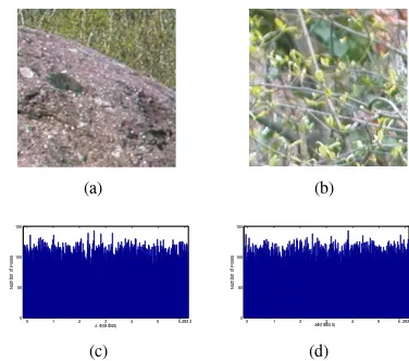
Not surprisingly, nature is replete with images exemplifying Definition 1. This, in turn, makes it possible to set up a naive image-based random number generator. To confirm this, we used more than70,000pairs of image patches of resolution
200×200randomly extracted from natural images [11]. For each pair, we computed∆φil and formulated the following null hypothesis
• H0:∀k∈ P ∆φil(k)∼U[0,2π).
which was tested using the Kolmogorov-Smirnov test [12]. For a significance level equal to 0.01, the null hypothesis was accepted for 94.05% of the image pairs with mean p-value equal to0.2848. In a similar setting, we tested Matlab’s random generator. The null hypothesis was accepted for
99.48%of the cases with meanp-value equal to0.501. Fig. 1 (a)-(b) show a typical pair of image patches considered in our experiment. Fig. 1 (c) and (d) plot the histograms of the gradient orientation differences and 40,000 samples drawn from Matlab’s random number generator respectively.
(a) (b)
0 1 2 3 4 5 6.2832
0 50 100 150
∆Φ(radius)
Number of Pixels
(c)
0 1 2 3 4 5 6.2832
0 50 100 150
∆Φ(radius)
Number of Pixels
[image:2.595.338.526.391.557.2](d)
Fig. 1. (a)-(b) An image pair used in our experiment, (c) Image-based random number generator: histogram of 40,000 gradient orientation differences and (d) Histogram of 40,000 samples drawn from Matlab’s random number generator.
IV. PCAOF GRADIENT ORIENTATIONS
A. Cosine-based correlation of gradient orientations
Given the set of our images{Ii}, we compute the
corre-sponding set of orientation images{Φi}and measure image
correlation using the cosine kernel
s(φi,φl),X k∈P
cos[∆φil(k)] =cN(P) (3)
wherec∈[−1,1]. Notice that for highly spatially correlated images∆φil(k)≈0 andc→1.
Assume that there exists a subsetP2⊂ P corresponding
we have
s1(φi,φl) = X
k∈P1
cos[∆φil(k)] =c1N(P1) (4)
where c1∈[−1,1].
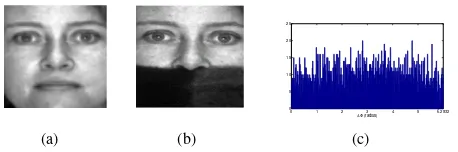
Not unreasonably, we assume that in P2, the images are
pixel-wise dissimilar according to Definition 1. For example, Fig. 2 (a)-(b) show an image pair whereP2is the part of the
face occluded by the scarf and Fig. 2 (c) plots the distribution of ∆φinP2.
(a) (b)
0 1 2 3 4 5 6.2832
0 5 10 15 20 25
∆Φ (radius) (c)
Fig. 2. (a)-(b) An image pair used in our experiments. (c) The distribution of∆φfor the part of face occluded by the scarf.
Before proceeding forP2, we need the following theorem.
Theorem II
Letu(.)be a random process andu(t)∼U[0,2π)then:
• E[R
Xcosu(t)dt] = 0 for any non-empty intervalX of
ℜ.
• Ifu(.)is mean ergodic, thenR
Xcosu(t)dt= 0.
Proof: Let us define the random process z(t) = cosu(t). Let alsofU(u) =U[0,2π)and we assumed thatu∼fU(u).
The integral s = Rb
az(t)dt of the stochastic process z(t)
is a random variables [12]. By interpreting the above as a Riemannian integral and using the linearity of the expectation operator, we conclude that
E{s} =Rb
aE{z(t)}dt= Rb
a
R+∞
−∞ cos(u)fU(u)du
=Rb a
R2π
0 cos(u)du= 0
(5)
which shows that the integralR
Xcosu(t)dtis equal to zero in
mean value. By further assuming mean-ergodicity, the time average is equal to the mean, thus we get
E(Z)∝
Z
z(t)dt≡
Z
X
cosu(t)dt= 0 (6)
which proves the Theorem.
We also make use of the following approximation
Z
X
cos[∆φil(t)]dt∝X
k∈P
cos[∆φil(k)] (7)
where with some abuse of notation, ∆φil is defined in the continuous domain on the left hand side of (7). Completely analogously, the above theorem and approximation hold for the case of the sine kernel.
Using the above results, forP2, we have
s2(φi,φl) = X
k∈P2
cos[∆φil(k)]≃0 (8)
It is not difficult to verify that ℓ2-based correlation i.e. the
inner product between two images will be zero if and only
if the images have interchangeably black and white pixels. Our analysis and (8) show that cosine-based correlation of gradient orientations allows for a much broader class of un-correlated images. Overall, unlikeℓ2-based correlation where
the contribution of outliers can be arbitrarily large,s(.) mea-sures correlation as s(φi,φl) = s1(φi,φl) +s2(φi,φl)≃
c1N(P1), i.e. the effect of outliers is approximately canceled
out.
B. The principal components of image gradient orientations
To show how (3) can be used as a basis for PCA, we first define the distance
d2(φi,φl) = p X
k=1
{1−cos[∆φil(k)]} (9)
We can write (9) as follows
d2(φi,φl) = 1 2
p X
k=1
{2−2 cos[φi(k)−φl(k)]}
= 1
2||e
jφi−ejφl||2 (10)
where ejφi = [ejφi(1), . . . , ejφi(p)]T. The last equality makes the basic computational module of our scheme ap-parent. We define the mapping from[0,2π)p onto a subset
of complex sphere with radiuspN(P)
zi(φi) =ejφi (11)
and apply linear complex PCA to the transformed datazi.
Using the results of the previous subsection, we can remark the following
Remark IIfP =P1∪ P2 with∆φil(k)∼U[0,2π), ∀k∈
P2, then Re[zHi zl]≃c1N(P1)
Remark IIIfP2=P, then Re[zHi zl]≃0 and Im[zHi zl]≃ 0.
Further geometric intuition about the mapping zi is
pro-vided by the chord between vectorszi andzl
crd(zi,zl) = q
(zi−zl)H(zi−zl) = p
2d2(φ
i,φl) (12)
Using crd(.), the results of Remark 1 and 2 can be refor-mulated as crd(zi,zl)≃
p
2((1−c1)N(P1) +N(P2))and
crd(zi,zl)≃ p
2N(P)respectively.
Overall, Algorithm 1 summarizes the steps of our PCA of gradient orientations.
Algorithm 1. Estimating the principal subspace
Inputs:A set of n orientation images Φi,i = 1, . . . , n of
ppixels and the numberk of principal components. Step 1.Obtainφi by writingΦi in lexicographic ordering.
Step 2. Compute zi = ejφi, form the matrix of the transformed dataZ= [z1| · · · |zn]∈ Cp×n and compute the
matrixT=ZHZ∈ Rn×n.
Step 3. Compute the eigen-decomposition ofT=UΛUH
and denote by Uk ∈ Cp×k and Λk ∈ Rk×k the
k−reduced set. Compute the principal subspace from
Bk =ZUkΛ
−1
2 k ∈ Cp
[image:3.595.63.292.245.321.2]Step 4.Reconstruct usingZ˜=BkBH kZ.
Step 5.Go back to the orientation domain usingΦ˜ =∠Z˜.
Let us denote byQ={1, . . . , n}the set of image indices and Qi any subset of Q. We can conclude the following
Remark III If Q = Q1∪ Q2 with zHi zl ≃ 0 ∀i ∈ Q2,
∀l ∈ Qand i6= l, then, ∃ eigenvector bl of Bn such that bl≃ N(1P)zi.
A special case of Remark III is the following
Remark IV If Q = Q2, then N(1P)Λ ≃ In×n and Bn ≃ 1
N(P)Z.
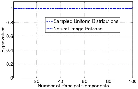
To exemplify Remark IV, we computed the eigen-spectrum of 100 natural image patches. In a similar setting, we computed the eigen-spectrum of samples drawn from Mat-lab’s random number generator. Fig. 3 plots the two eigen-spectrums.
20 40 60 80 100
0 0.2 0.4 0.6 0.8 1
Number of Principal Components
Eigenvalues
[image:4.595.64.284.307.449.2]Sampled Uniform Distributions Natural Image Patches
Fig. 3. The eigen-spectrum of natural images and the eigen-spectrum of samples drawn from Matlab’s random number generator.
Finally, notice that our framework also enables the direct embedding of new samples. Algorithm 2 summarizes the procedure.
Algorithm 2. Embedding of new samples
Inputs:An orientation imageΘofppixels and the principal subspaceBk of Algorithm 1.
Step 1.Obtainθ by writing Θin lexicographic ordering. Step 2. Compute z = ejθ and reconstruct using ˜z = BkBHkz.
Step 3.Go back to the orientation domain usingθ˜=∠˜z.
V. RESULTS
A. Face reconstruction
The estimation of a low-dimensional subspace from a set of a highly-correlated images is a typical application of PCA [13]. As an example, we considered a set of 50 aligned face images of image resolution 192×168 taken from the Yale B face database [14]. The images capture the face of the same subject under different lighting conditions. This setting usually induces cast shadows as well as other specularities. Face reconstruction from the principal subspace is a natural candidate for removing these artifacts.
We initially considered two versions of this experiment. The first version used the set of original images. In the sec-ond version, 20%of the images was artificially occluded by
a70×70“Baboon” patch placed at random spatial locations. For both experiments, we reconstructed pixel intensities and gradient orientations withℓ2intensiy-based PCA and PCA of
gradient orientations respectively using the first 5 principal components.
Fig. 4 and Fig. 5 illustrate the quality of reconstruction for 2 examples of face images considered in our experi-ments. While PCA-based reconstruction of pixel intensities is visually appealing in the first experiment, Fig. 4 (g)-(h) clearly illustrate that, in the second experiment, the reconstruction suffers from artifacts. In contrary, Fig. 5 (e)-(f) and (g)-(h) show that PCA-based reconstruction of gradient orientations not only reduces the effect of specularities but also reconstructs the gradient orientations corresponding to the “face” component only.
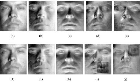
This performance improvement becomes more evident by plotting the principal components for each method and experiment. Fig. 6 shows the 5 dominant Eigenfaces of ℓ2
intensity-based PCA. Observe that, in the second experiment, the last two Eigenfaces (Fig. 6 (i) and (j)) contain “Baboon” ghosts which largely affect the quality of reconstruction. In contrary, a simple visual inspection of Fig. 7 reveals that, in the second experiment, the principal subspace of gradient orientations (Fig. 7 (f)-(j)) is artifact-free which in turn makes dis-occlusion in the orientation domain feasible.
Finally, to exemplify Remark III, we considered a third version of our experiment where 20% of the images were replaced by the same 192×168 “Baboon” image. Fig. 8 (a)-(e) and (f)-(j) illustrate the principal subspace of pixel intensities and gradient orientations respectively. Clearly, we may observe thatℓ2PCA was unable to handle the extra-class
outlier. In contrary, PCA of gradient orientations successfully separated the “face” from the “Baboon” subspace, i.e. no eigenvector was corrupted by the Baboon image (the “Ba-boon” orientation image appeared as a separate eigenvector). Note that the “face” principal subspace is not the same as the one obtained in versions 1 and 2. This is because only 80%
[image:4.595.318.554.576.726.2]of the images in our dataset was used in this experiment.
Fig. 5. PCA-based reconstruction of gradient orientations. (a)-(b) Orig-inal orientations used in version 1 of our experiment. (c)-(d) Corrupted orientations used in version 2 of our experiment. (e)-(f) Reconstruction of (a)-(b) with 5 principal components. (g)-(h) Reconstruction of (c)-(d) with 5 principal components.
Fig. 6. The 5 principal components of pixel intensities for (a)-(e) version 1 and (f)-(j) version 2 of our experiment.
Fig. 7. The 5 principal components of gradient orientations for (a)-(e) version 1 and (f)-(j) version 2 of our experiment.
B. Face recognition
PCA-based feature extraction for face recognition goes back to the classical work by Turk and Pentland [9] and still remains a standard benchmark for performance evaluation of new algorithms. We considered a single-sample-per-class experiment using aligned frontal-view face images taken
Fig. 8. (a)-(e) The 5 principal components of pixel intensities for version 3 of our experiment and (f)-(j) The 5 principal components of gradient orientations for the same experiment.
from the AR database [15]. The database consists of more than 4,000 frontal view facial images of 126 subjects. Each subject has up to 26 images taken in two sessions. The first session contains 13 images, numbered from 1 to 13, including different facial expressions (1-4), different lighting (5-7) and different occlusions under different lighting (8-13). The second session duplicated the first session two weeks later. We randomly selected a subset with 100 subjects. For training, we used 100 face images of 100 different subjects from session 1. We investigated the robustness of our scheme for the case of illumination variations and occlusions. In particular, we carried out the following experiments:
1) In experiment 1, we used the images 5-7 of session 2 for testing (different illumination).
2) In experiment 2, we used images 8-13 of session 2 for testing (occlusion by scarf or glasses under different illumination).
Note that the second experiment is very challenging since our single-sample-per-class training set does not allows us to find discriminant projection bases by exploiting class-label information, while the presence of the scarf or glasses in the testing set occludes approximately 25-40%of the total face area.
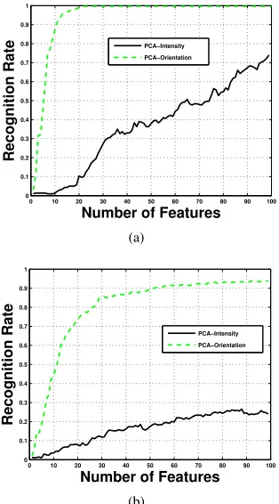
Table I and Fig. 9 summarize the results for our single sample per class experiments. The robustness of the proposed scheme is evident. As our results show, PCA of gradient orientations achieves almost 100% recognition rate for the case of illumination changes (experiment 1) and approx-imately 94% recognition rate for the case of occlusions (experiment 2). The latter result is approximately 20%better than the best reported recognition rate [18], which is obtained using as testing set a subset of the occluded images with
no illuminationvariations.
Moreover, the presented results should not be compared with those achieved by recent approaches such as the ones in [16] or [17] which use for training8 imagesper subject taken from both sessions, while the test images are also taken fromboth sessions(On the contrary, we used only
[image:5.595.56.296.330.471.2] [image:5.595.57.297.515.657.2]applied the method in [16] using
• features extracted using image resizing, intensity-based
PCA, LaplacianFaces as described in [16] for experi-ment 1.
• the robust extended ℓ1 minimization formulation for
experiment 2.
The third column of Table I shows the best results achieved by the method in [16]. As we may observe, our PCA of gradient orientations is not only significantly faster but also much more robust.
Recognition rate IGO-PCA I-PCA Best of [16]
Experiment 1 (illumination)% 99.67 74 74
[image:6.595.66.285.237.277.2]Experiment 2 (occlusions)% 94 28 32.33
TABLE I
RECOGNITION RESULTS ONARDATABASE FOREXPERIMENTS1AND2 (IGO-PCASTANDS FORPCAOFIMAGEGRADIENTORIENTATIONS
ANDI-PCASTANDS FORINTENSITY-BASEDPCA.
0 10 20 30 40 50 60 70 80 90 100
0 0.1 0.2 0.3 0.4 0.5 0.6 0.7 0.8 0.9 1
Recognition Rate
Number of Features
PCA−Intensity PCA−Orientation
(a)
0 10 20 30 40 50 60 70 80 90 100
0 0.1 0.2 0.3 0.4 0.5 0.6 0.7 0.8 0.9 1
Recognition Rate
Number of Features
PCA−Intensity PCA−Orientation
(b)
Fig. 9. Single sample per class face recognition experiment on the AR database. (a) Experiment 1 (illumination changes) (b) Experiment 2 (occlusions-illumination changes).
VI. CONCLUSIONS
We introduced a new concept: PCA of gradient orienta-tions. Our framework is as simple as standard ℓ2
intensity-based PCA, yet much more powerful for efficient subspace-based data representation. Central to our analysis is the distribution of gradient orientation differences and the cosine kernel which provide us a consistent way to measure image dissimilarity. We showed how this dissimilarity measure can
be naturally used to formulate a robust version of PCA. We demonstrated some of the favorable properties of our framework for the application of face recognition. Extensions of our scheme span a wide range of theoretical topics and applications; from statistical machine learning and clustering to object recognition and tracking.
REFERENCES
[1] N.A. Campbell,Robust procedures in multivariate analysis I: Robust Covariance estimation, Applied Statistics, 29 (1980), pp. 231–237. [2] C. Croux and G. Haesbroeck,Principal component analysis based on
robust estimators of the covariance or correlation matrix: influence functions and efficiencies, Biometrika, 87 (2000), pp. 603.
[3] Q. Ke and T. Kanade,Robust L1 norm factorization in the presence of outliers and missing data by alternative convex programming, in IEEE Computer Society Conference on Computer Vision and Pattern Recognition, CVPR (2005).
[4] N. Kwak,Principal component analysis based on L1-norm maximiza-tion, IEEE Transactions on Pattern Analysis and Machine Intelligence, 30 (2008), pp. 1672–1680.
[5] F.D.L. Torre and M.J. Black,A framework for robust subspace learn-ing, International Journal of Computer Vision, 54 (2003), pp. 117–142. [6] V. Chandrasekaran, S. Sanghavi, P.A. Parrilo and A.S. Willsky,
Rank-sparsity incoherence for matrix decomposition, preprint, (2009). [7] E.J. Candes, X. Li, Y. Ma, and J. Wright,Robust principal component
analysis?, Arxiv preprint arXiv:0912.3599, (2009).
[8] G. Tzimiropoulos, V. Argyriou, S. Zafeiriou, and T. Stathaki,Robust FFT-Based Scale-Invariant Image Registration with Image Gradients, IEEE Transactions on Pattern Analysis and Machine Intelligence, 32 (2010), pp. 1899–1906.
[9] M. Turk and A.P. Pentland, Eigenfaces for recognition, Journal of Cognitive Neuroscience, 3 (1991), pp. 71–86.
[10] A.J Fitch, A. Kadyrov, W.J. Christmas, and J. Kittler, Orientation correlation, in British Machine Vision Conference, 1 (2002), pp. 133– 142.
[11] H.P. Frey, P. Konig, and W. Einhauser,The Role of First and Second-Order Stimulus Features for Human Overt Attention, Perception and Psychophysics, 69 (2007), pp. 153–161.
[12] A. Papoulis and S.U. Pillai,Probability, random variables, and sto-chastic processes, McGraw-Hill New York (2004).
[13] M. Kirby and L. Sirovich,Application of the karhunen-loeve procedure for the characterization of human faces, IEEE Transactions Pattern Analysis and Machine Intelligence, 12 (1990), pp. 103–108. [14] A.S. Georghiades, P.N. Belhumeur and D.J. Kriegman,From few to
many: Illumination cone models for face recognition under variable lighting and pose, IEEE Transactions on Pattern Analysis and Machine Intelligence, 23 (2001), pp. 643–660.
[15] A.M. Martinez and R. Benavente,The AR face database, Tech. Rep., CVC Technical report (1998).
[16] J. Wright, A.Y Yang, A Ganesh, S.S. Sastry and Y. Ma,Robust face recognition via sparse representation, IEEE Transactions on Pattern Analysis and Machine Intelligence, 31 (2009), pp. 210–227. [17] Z. Zhou, A. Wagner, H. Mobahi, J. Wright and Y. Ma,Face recognition
with contiguous occlusion using Markov random fields, in Proceedings of International Conference on Computer Vision, ICCV (2009). [18] H. Jia, and A.M. Martinez,Face recognition with occlusions in the
training and testing sets, in Proc. Conf. Automatic Face and Gesture Recognition, FG(2008).
[19] X. Tan, S. Chen, Z.H. Zhou and F. Zhang, Recognizing partially occluded, expression variant faces from single training image per person with SOM and soft k-NN ensemble, IEEE Transactions on Neural Networks, 16 (2005), pp. 875–887.
[image:6.595.98.255.348.631.2]