R E S E A R C H
Open Access
A spanning tree construction algorithm for
industrial wireless sensor networks based
on quantum artificial bee colony
Yuanzhen Li
*, Yang Zhao and Yingyu Zhang
Abstract
In industrial Internet, many intelligent applications are implemented based on data collection and distribution. Data collection and data distribution in the wireless sensor networks are very important, where the node topology can be described by the spanning tree for obtaining an efficient transmission. Classical algorithms in graph theory such as the Kruskal algorithm or Prim algorithm can only find the minimum spanning tree (MST) in industrial wireless sensor networks. Swarm intelligence algorithm can obtain multiple solutions in one calculation. Multiple solutions are very helpful for improving the reliability of industrial wireless sensor networks.
In this paper, we combine quantum computing with artificial bee colony and design a spanning tree construction algorithm for industrial wireless sensor networks. Quantum computations are introduced into the onlooker bees search. Food source replacement strategy is improved. Finally, the algorithm is simulated and evaluated. The results show that the new proposed algorithm can obtain more alternative solutions and has a better performance in search efficiency.
Keywords:Industrial wireless sensor network, Minimum spanning tree, Artificial bee colony, Quantum computing
1 Introduction
WSN (wireless sensor networks) [1, 2] is an autono-mous measurement and control network system that consist of a large number of ubiquitous, small sensor nodes with communication and computing capabilities that are densely deployed in unattended monitoring areas [3]. WSN is a new information acquisition and processing technology [4]. Due to its advantages of low communication cost, flexible networking, and ease of use, it has a wide application prospect in the industry, military, environment, medical, and other fields [5]. IWSN (industrial wireless sensor networks) [6–8] is used to control and monitor various indus-trial tasks and is an emerging application of WSN.
Due to its high flexibility, low node cost, no wiring, and relatively easy maintenance, IWSN has been
fa-vored by more and more companies [9]. A large
number of wireless sensors are deployed in industrial parks [10]. These sensor nodes form a multi-hop net-work in the form of ad hoc netnet-works, which are very sensitive to the equipment, production lines, and en-vironmental information of the industrial site and transmitted to the control center in real time [11]. Through the calculation and analysis of data, the con-trol center can monitor the operating conditions of the equipment, find problems in a timely manner, issue control commands, and reduce safety problems in the production process.
IWSN faces more challenges than ordinary wireless sensor networks [12], which have the following fea-tures: (l) The sensor node deployment of the IWSN is related to the industrial environment. It needs to be manually installed on the plant equipment that
needs to be monitored [13], emphasizing reliable
monitoring of designated points [14]. The nodes of the WSN are generally deployed in a random and
© The Author(s). 2019Open AccessThis article is distributed under the terms of the Creative Commons Attribution 4.0 International License (http://creativecommons.org/licenses/by/4.0/), which permits unrestricted use, distribution, and reproduction in any medium, provided you give appropriate credit to the original author(s) and the source, provide a link to the Creative Commons license, and indicate if changes were made.
* Correspondence:[email protected]
dense manner, focusing on the overall coverage of the monitoring area. (2) In IWSN, once the sensor node is installed, it is generally no longer moving, unless the node failure needs to be replaced or the plant equipment is moved [15]; in contrast, the WSN node mobility is strong. (3) In addition to sensor nodes in IWSN, there are routers, handheld devices, and other nodes [16]. Different types of nodes perform different functions, forming a heterogeneous network. The WSN generally refers to homogeneous networks, and the status of nodes is equal. (4) The factory environ-ment is complex, and the interference is severe [17]. Therefore, the IWSN wireless network protocol de-sign aims at high reliability and real-time perform-ance. WSNs generally work in unattended areas. Node energy is limited, so the protocol design focuses on energy saving.
Field equipment production process data and
net-work status data are collected periodically [18].
IWSN analyzes and processes this data to monitor factory equipment and networks. In the production process, it is often necessary to obtain some statis-tical information, such as the total number of net-work nodes and the temperature of the production site [19]. At present, the data collection of industrial wireless networks is basically centralized. That is, the original data is uniformly collected and proc-essed by the central node. This is generally called the data collection protocol [20, 21]. The control formation such as commands for monitoring the in-dustrial field devices is performed through another protocol. This is generally referred to as data distri-bution protocol [22]. The data distribution process is one-to-many communication, and the data collection process is many-to-one communication. The above two processes are preferably implemented using trees to save network resources, especially the minimum spanning tree. Therefore, in industrial wireless sen-sor networks, how to construct an effective
mini-mum spanning tree (MST) is a critical issue [23].
Classical algorithms in graph theory, such as Kruskal algorithm and Prim algorithm, utilize greedy strat-egies to generate only one MST. In IWSN, a series of spanning trees are required to improve reliability
and deal with network changes [24]. Even if the
found spanning tree is not optimal, but suboptimal, the found suboptimal spanning tree has important practical significance for responding to the dynamic changes of the network.
In the evolutionary process of swarm intelligence algorithm [25–27], a series of solutions are gener-ated, which is very suitable for the solution of the spanning tree problem in Industrial Wireless Sensor Networks environment. At the same time, the swarm
intelligence optimization algorithm can search
without prior knowledge to find a solution to the optimization problem [28, 29]. Artificial bee colony algorithm is a kind of swarm intelligence algorithm, which was put forward by Karabogay in order to
solve the problem of multivariable function
optimization. Artificial bee colony algorithm is an optimization method proposed to imitate bee behav-ior. It is a specific application of swarm intelligence thought. Its main characteristic is that it does not need to know the special information about the problem, but only needs to compare the pros and cons of the problem. Through the local optimization behavior of individual artificial bees, the global opti-mal value is finally emerging in the group, and it has a faster convergence speed. Quantum computa-tion is a new computacomputa-tional model that follows quantum mechanics regulation to regulate quantum information units. From the point of view of compu-tational efficiency, due to the existence of the
super-position of quantum mechanics, some known
quantum algorithms are faster than conventional general-purpose computers when dealing with certain problems. In this paper, quantum computation and artificial bee colony algorithm are combined and a quantum artificial bee colony algorithm is proposed to solve multicast tree construction problem in indus-trial wireless sensor networks.
This paper is organized as follows: In Section 2, we first describe IWSN architecture and the minimum spanning tree problem in IWSN. We then present the proposed algorithm in Section 3. Sections 4 and 5 report the simulation results and discussion. Finally, Section 6 concludes the paper.
2 IWSN architecture and minimum spanning tree problem
Figure 1 shows the common IWSN architecture [30].
node information, and neighbor relationships, as well as the link status of the entire network. In addition,
the management server is also responsible for
processing network information, managing network
communication processes, and interacting with industrial applications. The security server [31] is responsible for the security management of the network and supports data integrity verification, data encryption, identity authentica-tion, and replay protection. The data server stores field de-vice configuration data, process flow data parameters, and data generated during the production process [32]. Gateways, management servers, security servers, and file servers are logically differentiated and can actually be deployed on the same network device as IWSNs controllers [33]. Finally, IWSN may need to connect to the Internet, depending on the specific conditions and needs of the factory.
A very important area of IWSN is data distribution and data collection. The effective implementation of data distribution and data collection is to use a minimal spanning tree. The minimum spanning tree problem is a basic problem in the areas of graph theory, optimization, and network optimization. Let graph G = (N,E,W) be a
connected undirected weighted graph, where N is the
set of nodes,E is the set of edges, and Wis the weight
defined on the edge. W ¼X
e∈E
we is the weight function.
In graph theory, a tree is defined as an acyclic connected graph. If a subgraph of a connected graph G is a tree and contains all vertices ofG, the subgraphTis called a spanning tree ofG. If Ghas nvertices, its spanning tree
has n vertices and n − 1 edges. WT¼
X
e∈ET
we is the
weight function of the tree T. The spanning tree of a graphGis not unique. A graph can have many different spanning trees. Among these trees, the spanning tree with the least sum of edge weight is the minimum span-ning tree (MST).
Because the minimum spanning tree problem is very important in network optimization, researchers have conducted a detailed study of this problem. At present, there are already some classical algorithms for solving the minimum spanning tree in graph the-ory, such as Kruskal algorithm or Prim algorithm. These algorithms can only get one solution at a time.
The characteristic of industrial wireless sensor
networks determines that multiple solutions are also necessary and meaningful. These different solutions are mutually complementary and backup. Swarm intelligence algorithm to obtain multiple solutions at a time just can effectively solve this requirement of industrial wireless sensor networks. This paper will use the artificial bee colony algorithm and use the idea of quantum computing to solve this problem.
3 Quantum artificial bee colony 3.1 Standard artificial bee colony
The artificial bee colony (ABC) algorithm [34],
originally proposed by Karaboga in 2005, is based on
the bee family’s foraging behavior. The bee is a
social insect. Although the behavior of individual
insects is extremely simple, the group of individuals shows extremely complex behavior. Bees can collect nectar from food sources with great efficiency in any environment; at the same time, they can adapt to changes in the environment. As a group organism of nature, the bee colony has a more rigorous foraging system within its organization. The artificial bee colony algorithm is based on the division of labor and cooperation of different types of work groups in the bee colony, thereby more effectively searching for the global optimal solution.
The minimum search model for swarms that generate swarm intelligence includes the basic three components
[35]: food sources, employed bees, and unemployed
bees. There are also two basic behavioral models: recruiting bees for food sources and giving up food sources. (1) Food sources: the value of food sources is determined by many factors, such as the distance from the hive, the richness of the nectar, and the ease of
obtaining nectar. (2) Employed bees: for each food source, there is only one employed bee, that is, the num-ber of employed bees is equal to the numnum-ber of food sources. The employed bee stores information about food sources and shares this information with other bees with a certain probability.(3) Unemployed bees: their main task is to find and mine food sources. There are two types of unemployed bees: the scout bees and the onlooker bees. Scout bees search for new food sources nearby. The onlooker bees wait inside the hive and find food sources by sharing information with the employed bee.
The ABC algorithm randomly generates initial
popula-tions containing PS solutions (food sources). The
employed bee conducts a neighborhood search on the corresponding food source, compares the new food source with the original food source, and selects a solution with a high degree of fitness as a candidate solution. When searching work finished, the employed bees share the food source information with the onlooker bees. The onlooker
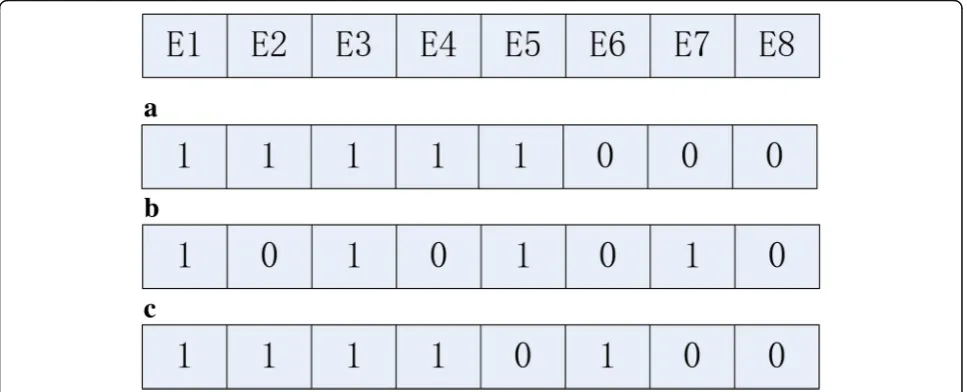
Fig. 3Example of binary coding. Binary coding is used to illustrate the coding techniques used in this paper
bees choose the food source according to probability pi. The higher the food source’s fitness value, the greater the probability of being selected.
pi¼ fi
XPS
i¼1
fi
ð1Þ
where fi is the fitness value of the i-th solution xi. Then, the onlooker bees also conduct a neighborhood search and choose a better solution. If a solution is not improved for consecutive NCcycles, it is discarded and a random solution is randomly generated by the scout bee. The main steps of the artificial bee colony algorithm are as follows.
(1) Initialize the colony population;
(2) Employed bees search for new honey source near their associated food sources;
(3) The onlooker bee to select the food source using formula (1) and search for a new honey source near the selected food source;
(4) Scout bees to search for new honey sources (5) Memorize the best food source found so far (6) If the maximum number of iterations is not reached, repeat the above steps (2–5). The final best honey position is the global optimal solution to be searched.
Artificial bee colony algorithm has shown good
performance [36, 37] in the solution of complex
optimization problems due to its advantages of simple principles, convenient implementation, good applicability, and favorable cooperation between population division and labor [38]. The original artificial bee colony algorithm is mainly aimed at solving the problem of continuous space function optimization. In order to solve many com-binatorial optimization problems in practical engineering, many discrete artificial bee colony algorithms are pro-posed. The flow of the discretized artificial bee colony algorithm is the same as the artificial bee colony algorithm.
3.2 Quantum artificial bee colony algorithm
Quantum computing is a new cross discipline com-bining information science and quantum mechanics. Quantum computations represented by quantum algo-rithms have a high degree of parallelism, exponential storage capacity, and exponential acceleration of clas-sical heuristic algorithms. It has great superiority and contains great vitality.
Quantum computing has become a frontier field for scholars from all over the world. By using quantum
computing in traditional intelligent optimization,
quantum computing and intelligent computing are com-bined. This will change the traditional optimization
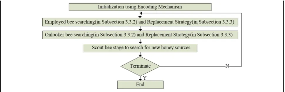
Fig. 5Flow chart of QABCST algorithm. The flow chart of the QABCST algorithm
methods of intelligent computing and improve the performance of search optimization and convergence speed. Using quantum computing to improve the par-ticle swarm algorithm, Sun et al. proposed quantum particle swarm optimization (QPSO) algorithm [39]. It is assumed that the particle’s behavior has quantum characteristics. Under the role of quantum mechanics, particles no longer have limitations on the trajectory and velocity, and the ability of particles to find the optimal solution is greatly improved. Regarding the specific implementation of the algorithm, QPSO uses (Eqs. 2–7) to update the entire population.
mb¼
XN
i¼1 pbi
N ð2Þ
a¼ randð0;1Þ ð3Þ
p¼apbiþð1−aÞ gb ð4Þ
b¼1− t
2tmax ð
5Þ
u¼ randð0;1Þ ð6Þ
pi¼
p−b jmb−pij ln 1
u ; u≥0:5
pþb jmb−pij ln 1
u ; u<0:5
8 > > < > >
: ð7Þ
Here, N is the population size; pbi is the individual
optimal position of the i-th particle; gb is the
optimal location of the entire population; mb is the mean of best position, which is the average of the individual optimal positions of all particles; rand(0,1) is a function whose return value is a random deci-mal between [0, 1]; t is the current evolutionary
gen-eration; tmax the maximum evolutionary generation
of the algorithm; b is called the contraction expan-sion coefficient, which gradually decreases with the iteration of the algorithm; pi is the position of the i -th particle.
Inspired by the QPSO algorithm, we use a similar
approach in the QABC (quantum artificial bee
colony) algorithm. We only use the idea of quantum computing in the onlooker stage. A quantum repre-sentation of solutions is used to enhance the diversity of the basic ABC. In addition, the exploitive capability of the ABC is boosted through the use of the quantum interference concept.
3.3 Quantum artificial bee colony algorithm for constructing spanning trees
3.3.1 Encoding mechanism
The standard ABC algorithm for solving continuous optimization problems is not directly suitable for solving the minimum spanning tree problem. Because the mini-mum spanning tree problem is an optimization problem, binary representation is used. The number of edges in the graph G is denoted as ∣E∣. ∣E∣ bit binary code is used to represent a solution. Each binary bit corresponds to an edge in the graph G and takes value 0 or 1, where 1 indicates that the corresponding edge is contained in the spanning tree T, and 0 means the opposite. The number of nodes in the graph G is denoted as∣N∣. Ac-cording to the characteristics of the spanning tree, the spanning tree contains only∣N∣ ‐1 edges. In a feasible solution, only ∣N∣‐1 binary bit is 1. The other binary bits are all 0. For example, given a graph, G = (N, E)
with |N| = 6 and |E| = 8 as shown in Fig. 2, where the edges and nodes are numbered in order so that each bit
of a solution could be decoded to an edge. Figure 3
shows three coding schemes. The corresponding graphs for the three coding schemes are shown in Fig. 4. The number of 1 in code (b) is 4, and (b) is an infeasible string. The number of 1 in code (a) and code (c) is 5. In Fig. 4, after decoding (c), there is a loop (v1-v2-v4-v1) and isolated node v5. Binary string (a) is a feasible code; binary string (c) is not an infeasible code.
3.3.2 Search mechanism
In the initialization phase, for each food source, |N| − 1 position is randomly selected and set to1and other posi-tions are set to0. The calculation of fitness is calculated ac-cording to formula (8). If the binary string is a feasible code (Figs.3aand4a), the fitness value isfit¼X
e∈ET
we. If the
bin-ary string is infeasible (Figs.3cand4c), the fitness is∞.
fit¼
Employed bees use the following techniques when searching. A position is randomly chosen from the elements with 1 and denoted as i1. Another position is randomly chosen from the elements with 0 and denoted as i2. The values of positions i1and i2are interchanged. After such changes, the number of elements with 1 does not change. This technique can guarantee that the num-ber of 1 in the binary string is constant. The fitness of the newly generated solution is calculated according to Eq. (8). The replacement strategy, described in detail in Section 3.3.3, is executed.
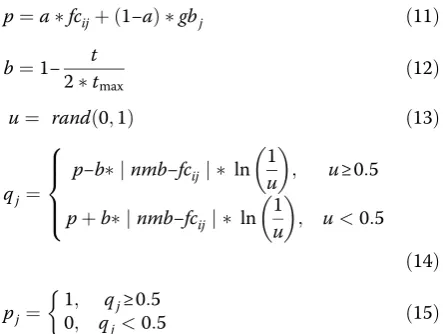
In the process of onlooker bee searching, the quantum computing technique introduced in Section 3.2 is used and improved. For the calculation of the average best position, we use the elite strategy. Food sources are sorted in order of fitness value from small to large. For the sorted food source, the mean value of the front half food source is calculated (for-mula (9)). Because the particle swarm algorithm and the artificial bee swarm algorithm are essentially dif-ferent, the meaning of the variable has also changed. In order to apply to the artificial bee colony algo-rithm, the previous formulas (2)–(7) are modified. The new calculation methods are formulas (9)–(15).
nmbj¼
Table 1The coordinates of the nodes
Node X Y Node X Y V1 40.94 292.97 V9 309.2 1.1. 320.0 V2 75.53 226.48 V10 277.73 1.2. 55.13 V3 141.22 329.18 V11 308.81 1.3. 222.7 V4 230.90 377.83 V12 419.35 1.4. 254.59 V5 135.32 160.54 V13 343.43 1.5. 150.27 V6 189.61 272.43 V14 365.85 1.6. 43.24 V7 192.76 94.59 V15 464.2 1.7. 177.83 V8 244.29 204.32 V16 145.33 1.8. 93.51
Table 2The weight of the edges
p¼afcijþð1−aÞ gbj ð11Þ
Here,Nis the population size;fcijis thej-th component of the i-th smallest food source according to fitness;gb is the first small food source according to fitness; gbj is the j-th component of gb; nmb is the mean after improvement; Rand(0, 1) is a function whose return value is a random deci-mal between [0, 1];tis the current evolutionary generation; tmaxthe maximum evolutionary generation of the algorithm;
bis called the contraction expansion coefficient, which grad-ually decreases with the iteration of the algorithm.
Ifpjand thej-th component of the current food source are equal, nothing is done. Otherwise, a location, denoted ask, is randomly selected from the elements with (1−pj). Then, the elements of position kand positionj are inter-changed. That is, the element at position jis assigned pj, and the element at positionkbecomes 1 −pj. The above operation is the same as the operation of the employed bee, and it also ensures that the number of elements with 1 does not change. The search process for onlooker bees is shown in Algorithm 1.
If no better food source is found in the search for employed bees and onlooker bees, the food source is not updated. If it is not updated after the set number of times,
the food source is discarded. The scout bee will randomly generate a new food instead. The procedure is similar to the initialization step.
3.3.3 Replacement strategy
In the previous part of this article, we have mentioned that multiple solutions can be obtained in one calcula-tion. Therefore, the first principle of our replacement strategy is to ensure the diversity of food sources. Under the guidance of such principles, if the newly found food source is better than the original food source, but is the same as any other food source, it will not be updated and will be discarded. In addition, as described in Sec-tion 3.3.1, the initial food source and new food source search may be infeasible. Therefore, another principle of our replacement strategy is to replace as much of the in-feasible food source as possible.
After employed bee and onlooker bees search for new food sources, the specific algorithm for food source replacement is shown in Algorithm 2.
To this position in this paper, based on quantum com-puting and artificial bee colony, the algorithm for solving the spanning tree of industrial wireless sensor networks has been introduced. We will use QABCST to represent this algorithm later. The main steps of QABCST are simi-lar to the ABC algorithm described in Section 3.1. The flow chart of the QABCST algorithm is shown in Fig.5.
The QABCST algorithm can generate multiple solu-tions in one calculation, and these solusolu-tions are backups of each other. The tree decoded from optimal solution can be used for data distribution or data collection. When the link failure causes the optimal tree to be un-available, one of the backup solutions is used. Firstly, the
Table 3Minimum spanning tree found by the Kruskal algorithm
ST Weight Edge series
candidate solutions containing the failed link can be marked as invalid. Then, choose the optimal one from the remaining solutions.
4 Experimental
In this section, simulation experiments are conducted on the newly proposed algorithm to verify the validity of our proposed algorithm.
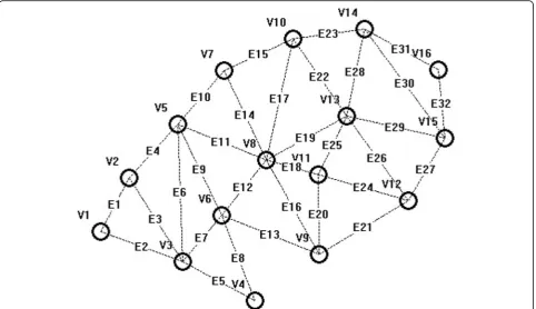
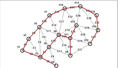
The industrial wireless sensor network shown in
Fig. 6 is used as an example to simulate. The
Fig. 7Minimum spanning tree found by the Kruskal algorithm. The minimum spanning tree obtained by the Kruskal algorithm during performance simulation
Table 4Spanning tree found by BABC
ST Weight Edge series
1 1431.365601 1,7,8,10,11,15,18,20,24,25,27,28,29,31,32 2 1505.983398 1,3,5,7,10,12,13,15,18,23,24,28,30,31,32 3 1452.080566 1,4,5,7,8,10,13,18,23,24,25,26,27,28,31 4 1595.697266 2,4,7,8,9,10,12,16,17,19,20,21,22,23,32 5 1447.339722 1,2,5,7,9,10,18,19,20,23,25,26,27,28,31 6 1423.100586 1,2,5,7,8,10,12,15,18,20,21,23,27,28,31 7 1501.466919 1,7,8,9,10,15,17,18,20,23,24,26,27,28,32 8 1424.996460 1,5,7,10,15,18,19,20,21,23,24,25,26,27,32 9 1465.025146 2,4,8,9,10,12,13,14,15,18,23,25,27,31,32 10 1449.954712 1,2,4,5,7,10,12,16,19,22,25,27,28,31,32 Optimal solution 1326.409668 1,2,4,5,7,10,12,15,18,20,23,25,27,31,32
Table 5Spanning tree found by QABCST
ST Weight Edge series
industrial wireless sensor network, represented as G, has 16 nodes and 32 edges. These nodes are deployed
in a 500 × 400 rectangular area. Table 1 shows the
coordinates of the nodes.The weight function on each edge is the Euclidean distance between two nodes.
Table 2 lists the correspondence between edges and
nodes, as well as the weight of the edges.
Our new proposed algorithm will be compared with
Kruskal algorithm and BABC [40] algorithm. BABC
uses the basic artificial bee colony algorithm to solve the minimum spanning tree. It can also obtain mul-tiple spanning tree construction schemes in one cal-culation. The population size is 20, and the algorithm loops 3000 times. All the algorithms have been coded using C++ in VS 2010. We run all the configurations on an Intel (R) Core (TM) i7-2600 CPU @ 3.40 GHz with 8.00 GB RAM in the Windows 10 Operation System.
5 Results and discussion
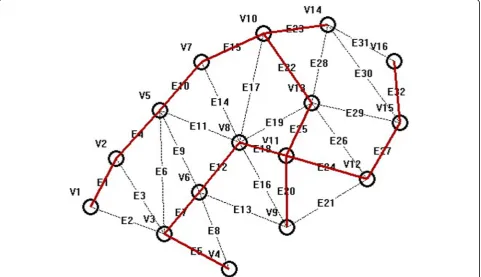
Each of the three algorithms runs one time, and the experimental results are compared. First, the Kruskal algorithm is used to handle this example. The Kruskal algorithm can only obtain one solution. The obtained ST (spanning tree) is shown in Table 3. The resulting spanning tree has a weight of 1326.409668. The
resulting minimum spanning tree is shown in Fig. 7.
The Kruskal algorithm’s calculation time is about
0.05 s.
Tables 4 and 5 are the results obtained after the
BABC and QABCST algorithms are run once. As can
be seen from Tables 4 and 5, the QABCST algorithm
has got more solutions. This is due to the diversity of our replacement strategies. The reason for this result is the persistence of diversity in QABCST’s replace-ment strategy. Figure 8 is an illustration of the other one (10th in Table 5) of the solutions obtained by the QABCST algorithm.
The following is a comparison of the average performance of the QABCST and BABC algorithms running multiple times. The algorithm is performed 10 times independently to obtain its average
perform-ance. Table 6 shows the average of the 10 minimum
spanning tree weights. The result of Table 6 about
Kruskal is the result of running once. As can be seen from the table, the QABCST algorithm has better per-formance than BABC.
Table 6Average of the 10 minimum spanning tree weights
Kruskal BABC QABCST 1326.409668 1328.747522 1327.755135
6 Conclusion
With the rapid development of wireless sensor networks, wireless devices are increasingly deployed in industrial environments. Compared with common wireless sensor networks, industrial wireless sensor networks have higher requirements for the determinism and reliability of data communications. Therefore, it is particularly im-portant to design reasonable mechanisms for the data aggregation/distribution of IWSNs to ensure the cer-tainty and reliability of the data transmission process. Data collection and distribution in industrial wireless sensor networks can be described using the spanning tree problem in graph theory. Existing classical algo-rithms such as Kruskal and Prim algorithm can only get one solution at a time. In order to improve reliability, in-dustrial application scenarios need to provide multiple solutions for mutual backup. This paper improves the artificial bee colony algorithm based on the idea of quantum computing and proposes a spanning tree con-struction algorithm for industrial wireless sensor net-works based on quantum artificial bee colony. Finally, our algorithm was verified by experiments. The experi-mental results show that the algorithm can achieve bet-ter performance and can obtain more solutions at the same time. Future work includes increasing a priori knowledge of the network structure to improve search efficiency.
Abbreviations
MST:Minimum spanning tree; WSN: Wireless sensor networks; IWSN: Industrial wireless sensor networks; ABC: Artificial bee colony; QPSO: Quantum particle swarm optimization; QABC: Quantum artificial bee colony; ST: Spanning tree
Acknowledgements
Not applicable.
Authors’contributions
The first author conducted the experiments and wrote the first draft of the paper. Other co-authors helped to revise the paper and polished the paper. All authors read and approved the final manuscript.
Authors information
Not applicable.
Funding
This research was supported by National Natural Science Foundation of China (No. 61773192).
Availability of data and materials
Not applicable.
Competing interests
The authors declare that they have no competing interests.
Received: 5 July 2018 Accepted: 24 June 2019
References
1. H. Cheng, Z. Su, N. Xiong, Y. Xiao, Energy-efficient node scheduling algorithms for wireless sensor networks using Markov random field model. Inf. Sci329(C), 461–477 (2016)
2. X. Jiang, Z. Fang, N.N. Xiong, et al., Data fusion-based multi-object tracking for unconstrained visual sensor networks. IEEE. Access.6, 13716–13728 (2018)
3. J. Liu, J. Wan, Q. Wang, P. Deng, K. Zhou, Y. Qiao, A survey on position-based routing for vehicular ad hoc networks. Telecommun. Syst.62(1), 15– 30 (2016)
4. M. Wu, L. Tan, N. Xiong, Data prediction, compression, and recovery in clustered wireless sensor networks for environmental monitoring applications. Inf. Sci.329(SI), 800–818 (2016)
5. Y. Liu, K. Ota, K. Zhang, et al., QTSAC: an energy-efficient MAC protocol for delay minimization in wireless sensor networks. IEEE Access.6, 8273–8291 (2018) 6. V. C G, G. P H, Industrial wireless sensor networks: challenges, design
principles, and technical approaches. IEEE Trans. Ind. Electron.56(10), 4258– 4265 (2009)
7. D.E. Boubiche, A.S. Pathan, J. Lloret, H. Zhou, S. Hong, S.O. Amin, M.A. Feki, Advanced industrial wireless sensor networks and intelligent IoT. IEEE. Commun. Mag56(2), 14–15 (2018)
8. D.V. Queiroz, M.S. Alencar, R.D. Gomes, I.E. Fonseca, C. Benavente-Peces, Survey and systematic mapping of industrial wireless sensor networks. J. Netw. Comput. Appl.97, 96–125 (2017)
9. M. Gidlund, S. Han, E. Sisinni, A. Saifullah, U. Jennehag, From industrial wireless sensor networks to industrial Internet of things. IEEE. Trans. Ind. Inf.
14(5), 2194–2198 (2018)
10. T. Liang, B. Zeng, J. Liu, L. Ye, C. Zou, An unsupervised user behavior prediction algorithm based on machine learning and neural network for smart home. IEEE. Access.6, 49237–49247 (2018)
11. J. Liu, J. Wan, B. Zeng, Q. Wang, H. Song, M. Qiu, A scalable and quick-response software defined vehicular network assisted by mobile edge computing. IEEE. Commun. Mag.55(7), 94–100 (2017)
12. Cheffena, industrial wireless sensor networks: channel modeling and performance evaluation. EURASIP. J. Wirel. Commun. Netw.297(2012) 13. C. Wang, J. Li, B. Wang, Face synthesis based on parts-based sparse
component analysis face representation. Optik. Int. J. Light. Electron. Opt
140, 843–852 (2017)
14. M. Kumar, R. Tripathi, S. Tiwari, QoS guarantee towards reliability and timeliness in industrial wireless sensor networks. Multimed. Tools. Appl.
77(4), 4491–4508 (2018)
15. S. Wu, W. Chou, J. Niu, M. Guizani, Delay-aware energy-efficient routing towards a path-fixed mobile sink in industrial wireless sensor networks. SENSORS.18(3), 899 (2018)
16. J. Tan, A. Liu, M. Zhao, H. Shen, M. Ma, Cross-layer design for reducing delay and maximizing lifetime in industrial wireless sensor networks. EURASIP J. Wirel. Commun. Netw.50(2018)
17. M. Huang, A. Liu, N.N. Xiong, et al., A low-latency communication scheme for mobile wireless sensor control systems. IEEE. Trans. Syst. Man. Cybern. Syst.49(2), 317–332 (2019)
18. W. Zhang, J. Chang, F. Xiao, et al., Design and analysis of a persistent, efficient, and self-contained WSN data collection system. IEEE. Access.7, 1068–1083 (2019)
19. J. Tan, W. Liu, T. Wang, et al., An adaptive collection scheme-based matrix completion for data gathering in energy-harvesting wireless sensor networks. IEEE. Access.7, 6703–6723 (2019)
20. H. Zheng, W. Guo, N. Xiong, A Kernel-based compressive sensing approach for mobile data gathering in wireless sensor network systems. IEEE. Trans. Syst. Man. Cybern. Syst.48(12), 2315–2327 (2018)
21. X. He, S. Liu, G. Yang, et al., Achieving efficient data collection in heterogeneous sensing WSNs. IEEE. Access.6, 63187–63199 (2018) 22. K. Huang, Q. Zhang, C. Zhou, N. Xiong, Y. Qin, An efficient intrusion
detection approach for visual sensor networks based on traffic pattern learning. IEEE Trans. Syst. Man. Cybern. Syst.47(10), 2704–2713 (2017) 23. H. Cheng, Y. Chen, N. Xiong, et al., Layer-based data aggregation and
performance analysis in wireless sensor networks. J. Appl. Math.502381(2013) 24. S. Montero, J. Gozalvez, M. Sepulcre, Neighbor discovery for industrial
wireless sensor networks with mobile nodes. Comput. Commun.111, 41–55 (2017)
25. Z. Zheng, J. Li, Optimal chiller loading by improved invasive weed optimization algorithm for reducing energy consumption. Energ. Buildings.
161, 80–88 (2018)
26. J. Li, Q. Pan, S. Xie, An effective shuffled frog-leaping algorithm for multi-objective flexible job shop scheduling problems. Appl. Math. Comput.
27. H. Sang, Q. Pan, J. Li, et al., Effective invasive weed optimization algorithms for distributed assembly permutation flowshop problem with total flowtime criterion. Swarm. Evol. Comput.44(6), 64–73 (2019)
28. Z. Zheng, J. Li, P. Duan, Optimal chiller loading by improved artificial fish swarm algorithm for energy saving. Math. Comput. Simul.155(SI), 227–243 (2019) 29. H. Sang, Q. Pan, P. Duan, et al., An effective discrete invasive weed
optimization algorithm for lot-streaming flowshop scheduling problems. J. Intell. Manuf.29(6), 1337–1349 (2018)
30. J. Zhao, Y. Qin, D. Yang, J. Duan, Reliable graph routing in industrial wireless sensor networks. Int. J. Distrib. Sens. Netw.9(12), 758217 (2013)
31. J. Akerberg, M. Gidlund, T. Lennvall, J. Neander, M. Bjorkman, Efficient integration of secure and safety critical industrial wireless sensor networks. EURASIP. J. Wirel. Commun. Netw.100(2011)
32. J. Li, P. Duan, H. Sang, et al., An efficient optimization algorithm for resource-constrained steelmaking scheduling problems. IEEE. Access.6, 33883–33894 (2018)
33. C. Pei, Y. Xiao, W. Liang, X. Han, Trade-off of security and performance of lightweight block ciphers in Industrial Wireless Sensor Networks. EURASIP. J. Wirel. Commun. Netw.117(2018)
34. J. Li, Q. Pan, P. Duan, An improved artificial bee colony algorithm for solving hybrid flexible flowshop with dynamic operation skipping. IEEE. Trans. Cybern.46(6), 1311–1324 (2016)
35. K.Z. Gao, P.N. Suganthan, Q.K. Pan, et al., Artificial bee colony algorithm for scheduling and rescheduling fuzzy flexible job shop problem with new job insertion. Knowl. Based. Syst.109, 1–16 (2016)
36. Y.Y. Han, Q.K. Pan, J.Q. Li, et al., An improved artificial bee colony algorithm for the blocking flowshop scheduling problem. Int. J. Adv. Manuf. Technol.
60, 1149–1159 (2012)
37. Y. Han, J.J. Liang, Q. Pan, et al., Effective hybrid discrete artificial bee colony algorithms for the total flowtime minimization in the blocking flowshop problem. Int. J. Adv. Manuf. Technol.67, 397–414 (2013)
38. J. Li, Q. Pan, Solving the large-scale hybrid flow shop scheduling problem with limited buffers by a hybrid artificial bee colony algorithm. Inf. Sci.316, 487–502 (2015)
39. Jun S, Wenbo X, Bin F, in Proceedings of 2005 IEEE International Conference on Systems, Man and Cybernetics. Adaptive parameter control for quantum-behaved particle swarm optimization on individual level (IEEE 2005), pp. 3049-3054.
40. X. Zhang, X. Zhang, A binary artificial bee colony algorithm for constructing spanning trees in vehicular ad hoc networks. Ad. Hoc. Networks.58(4), 198– 204 (2017)
Publisher’s Note