FULL PAPER
3-D inversion of magnetic data based
on the L1–L2 norm regularization
Mitsuru Utsugi
*Abstract
Magnetic inversion is one of the popular methods to obtain information about the subsurface structure. However, many of the conventional methods have a serious problem, that is, the linear equations to be solved become ill-posed, under-determined, and thus, the uniqueness of the solution is not guaranteed. As a result, several different models fit the observed magnetic data with the same accuracy. To reduce the non-uniqueness of the model, con-ventional studies introduced regularization method based on the quadratic solution norm. However, these regulari-zation methods impose a certain level of smoothness, and as the result, the resultant model is likely to be blurred. To obtain a focused magnetic model, I introduce L1 norm regularization. As is widely known, L1 norm regularization promotes sparseness of the model. So, it is expected that, the resulting model is constructed only with the features truly required to reconstruct data and, as a result, a simple and focused model is obtained. However, by using L1 norm regularization solely, an excessively concentrated model is obtained due to the nature of the L1 norm regulariza-tion and a lack of linear independence of the magnetic equaregulariza-tions. To overcome this problem, I use a combinaregulariza-tion of L1 and L2 norm regularization. To choose a feasible regularization parameter, I introduce a regularization parameter selection method based on the L-curve criterion with fixing the mixing ratio of L1 and L2 norm regularization. This inversion method is applied to a real magnetic anomaly data observed on Hokkaido Island, northern Japan and reveals the subsurface magnetic structure on this area.
Keywords: L1–L2 norm regularization, 3D magnetic inversion, Lasso, Elastic net
© The Author(s) 2019. This article is distributed under the terms of the Creative Commons Attribution 4.0 International License (http://creat iveco mmons .org/licen ses/by/4.0/), which permits unrestricted use, distribution, and reproduction in any medium, provided you give appropriate credit to the original author(s) and the source, provide a link to the Creative Commons license, and indicate if changes were made.
Introduction
The inversion of geomagnetic field data has been consid-ered by many studies that aim to determine the property and geometry of subsurface magnetic structures. One of the major approaches is magnetic property inversion, which automatically retrieves the distribution of sub-surface magnetization or magnetic susceptibility from observed magnetic data. In these studies, the subsurface space is divided into a number of small grid cells assum-ing the susceptibility of each grid cell is homogeneous. In this situation, the equation to be solved becomes lin-ear and the susceptibility of each cell is obtained by the inversion minimizing a specific model objective function.
The main problem of this approach is the ambiguity of the solution caused by the inherent non-uniqueness
of the potential field. Furthermore, in the case of the 3D magnetic inverse problem, this ambiguity is emphasized because the problem is ill-posed in most cases. Accord-ingly, it is possible for several different models to fit the observed magnetic data with the same accuracy.
One promising mathematical approach to overcome this difficulty is to use an appropriate regularization method. Regularization is, simply speaking, a method to restrict the model space in which we seek the solution to a subspace of a specific class of models that have desig-nated characteristics.
For magnetic and the other geophysical inverse prob-lems, one of the traditional regularization methods is Tikhonov regularization (Tikhonov and Arsenin 1977). In this method, to reduce the ambiguity of the prob-lem and to stabilize the solution, a quadratic penalty related to the solution norm is introduced into the objec-tive function. Li and Oldenburg (1996) used L2 and first-order spatial differentiation norm as the penalty.
Open Access
*Correspondence: [email protected]
Pilkington (1997) introduced a (depth weighted) L2 norm penalty for magnetic inversion. In the electromagnetic studies, for example, Minami et al. (2018) introduced a smoothness penalty into the 3D resistivity inversion and succeeded in detecting the temporal change of the subsurface resistivity structure related to the volcanic activities. Furthermore, Tikhonov regularized inverse problems have been often solved within the framework of the Bayesian approach in the field of the magnetic (e.g., Zeyen and Pous 1991; Tsunakawa et al. 2010; Honsho et al. 2012) and electromagnetic studies (e.g., Ogawa and Uchida 1996). These studies show that the stability and the robustness of the solution are improved. However, because the quadratic solution norm penalty imposes a certain level of smoothness on the model (Hansen 1992), the obtained model tends to be blurred and unfocused. Especially in the case of the magnetic inversion, such blurred feature sometimes makes it look geologically unrealistic.
To obtain a focused model, some studies introduced sparsity regularization which promotes the so-called sparseness into the model. Last and Kubik (1983) intro-duced a minimum-support penalty into gravity inversion to recover sharp boundaries of the subsurface density structure. Portniaguine and Zhdanov (1999, 2002), and Zhdanov et al. (2004) proposed 3D focusing magnetic data and gravity gradiometry data inversion, introducing a minimum support, or minimum gradient support pen-alty. Zhdanov et al. (2000, 2000), Zhang et al. (2015), and Xiang et al. (2017) also introduced minimum gradient support into electromagnetic inversion to recover a resis-tivity structure with sharp boundaries. Pilkington (2009) proposed to use a Cauchy norm penalty (Sacchi and Ulrych 1995) for 3D magnetic inversion. A Cauchy norm penalty has also been used in some recent 3D magnetic and gravity inversion studies (e.g., Uieda and Barbosa 2012; Abedi et al. 2015; Wang et al. 2015; Rezaie et al. 2016). These penalties realize sparseness of the model by minimizing the number of non-zero components of the model, or the gradient of the model. In simulation stud-ies with synthetic data, these studstud-ies demonstrated that a model very close to the true model can be reconstructed and showed the effectiveness of sparse regularization for the potential inverse problem. This fact means that the sparse regularization reduced the ambiguity due to the non-uniqueness of the potential field and the ill-posed-ness of the problem and provided a focused model with high resolution.
For the sparse regularization, Tibshirani (1996) pro-posed an L1 norm regularization method named LASSO (least absolute shrinkage and selection operator) in a statistical study. L1 norm regularization minimizes an objective function which contains a penalty based on
the L1 norm of the solution vector. This regularization method is known to have a tendency to choose a sparse model and has, therefore, been immensely popular in various research fields in recent years. In geophysical research, L1 norm regularization has also been used, for example, in seismic tomography studies (e.g., Loris et al. 2007; Wang 2011; Fang and Zhang 2014; Liu et al. 2015).
The basic idea of sparse regularization is L0 norm minimization which is to limit the number of non-zero model elements to a minimum. However, the L0 norm problem is not convex, and it is known that, this problem is NP-hard, and no trivial method to solve this problem efficiently has been found. Therefore, in general, the L0 norm problem is replaced by an alternative convex prob-lem by relaxing the constraints of the solution. The regu-larized inversion using minimum support and Cauchy norm is one of these alternative convex problems, and L1 norm regularization is also one of such alternative problems.
In this paper, a new sparse magnetic inversion method based on L1 norm regularization is proposed. However, for this purpose, we have to address some specific prob-lems of magnetic data inversion. One problem is the lack of depth resolution due to the rapid decay of the magnetic field. As a consequence, an unrealistic model which is excessively concentrated in the shallow region is likely to be provided by magnetic inversion. To tackle this problem, an appropriate weighting function which counteracts the field decay has to be introduced. In con-ventional studies, Li and Oldenburg (1996) proposed a depth weighting function and Li and Oldenburg (2000) used a sensitivity-based weighting function. On the other hand, Tibshirani (1996) dealt with a normalized regres-sion problem that is equivalent to using the square of the sensitivity-based weighting function of Li and Oldenburg (2000). In this paper, some synthetic tests are performed and the most suitable weighting function for L1 norm regularized magnetic inversion is discussed.
Another problem is that, magnetic data inversion is an under-determined problem in most cases, that is, the num-ber of observations (N) is much lower than the number of unknown model parameters (M). In such an N <<M
on an L-curve criterion with fixing the mixing ratio of L1 and L2 norm regularization, a priori. In this paper, the effectiveness of the proposed inversion method as well as the parameter selection methods are discussed through some synthetic tests and real field data.
Observation equations
By assuming that there is no remanent magnetization, and induced magnetization is dominant in our study area, mag-netization distribution in the volume V is written as
where H0 is the Earth’s geomagnetic field, and the vector
l is an unit-vector parallel to H0 . κ(r′) and β∗(r′) are the susceptibility and the intensity of the induced magneti-zation on r′∈V , respectively. The total magnetic field F resulting from this induced magnetization can be written as a Fredholm integral equation:
where µ0 is the magnetic permeability of vacuum, r ∈V is the observation point, and ∇r and ∇r′ are the gradient operators with respect to r and r′ , respectively. ||r−r′|| is the Euclidean distance between r and r′:
To solve the integral equation of Eq. (1) numerically,
V is divided into a 3D grid of rectangular block cells (�V1,. . .,�VM) . Now, let us denote the magnetic total field produced by a grid cell Vj with unit induced mag-netization by
Supposing the susceptibility in each grid cell is con-stant, the magnetization also becomes concon-stant, that is, β∗(r′j)=βj∗ for r′j∈Vj . Then, Eq. (1) is rewritten as
When we have a data set of a magnetic anomaly observed
on (r1,. . ., rN) , Eq. (1) can be discretized as
This equation can be rewritten in vector-matrix form: β∗(r′)l=κ(r′)H0, vided by Bhattacharyya (1964). The j-th column vector of K , kj , is the total field over the discrete observation points (r1,. . ., rN) produced by Vj with unit induced magnetization.
In order to obtain magnetic structure with high resolu-tion, it is necessary to finely subdivide V in the lateral direc-tions as well as the depth direction. Consequently, in most cases, the number of grid cells M exceeds the number of the observation points N and the magnetic inverse prob-lem of Eq. (3) becomes an under-determined and ill-posed problem, which means a unique solution does not exist. A conventional way to solve such an ill-posed problem is to rely on regularization methods. In a regularization method, the problem to be solved is replaced by the minimization of the following objective function:
where P(β∗) is a penalty function and the constant (>0) is a regularization parameter that controls the strength of the penalty. The explicit form of P differs according to each regularization method, and each method provides different qualities in the solution.
Further, in conventional studies of magnetic inversion, a weighting procedure is commonly introduced into the pen-alty. Because the amplitude of the total field kj produced by the deeper cells decays rapidly, it is not sensitive to the data. Thus, the resultant model tends to concentrate strongly on a very shallow region. In order to compensate for this ten-dency, we have to introduce a weighting in the penalty to counteract the magnetic field decay:
where W is a diagonal matrix
where βˆ is a solution which minimizes Eq. (7). Finally, the susceptibility model is obtained by
Weighting function
For the weighting function of Eq. (6), Li and Oldenburg (2000) introduced sensitivity-based weighting defining the integrated sensitivity of matrix K:
They introduced the following sensitivity-based weight-ing function to reduce the disparity in the sensitivities of each column of K:
Li and Oldenburg (2000) and Portniaguine and Zhdanov (2002) used this function with γ =1 as the weighting function:
Alternatively, LASSO proposed by Tibshirani (1996) deals with a normalized regression problem, that is, each column vector kj is assumed to be normalized. Obvi-ously, this data setting is equivalent to using the weight-ing of Eq. (8) with γ =2:
In the later section, some synthetic tests are performed and we discuss the performance of the above weighting functions.
L1 norm regularization
L1 norm regularization minimizes an objective function L which involves an L1 norm penalty of the solution vector β:
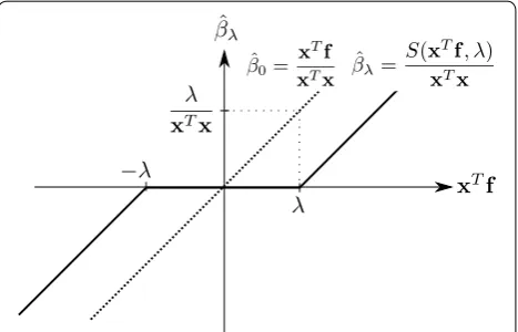
By introducing the L1 norm penalty, sparseness of the model is promoted. To see how the L1 norm regulariza-tion introduces the sparseness into the model, consider the following simplified single-variable problem. Sup-pose that the matrix X has only one column, that is, X is
where a superscript T indicates the transpose. Thus, the β that minimizes Eq. (12) is obtained as
However, because we are now considering the case of β >0 , this yields the following result:
By similar calculation in the case of β <0 , we can obtain the following integrated result:
where S is the following soft-thresholding operator:
The plot of Eq. (13) is shown in Fig. 1. The solid line shows ˆ
β of Eq. (13). The dashed line indicates βˆ0=xTf/xTx which is Eq. (13) with =0 , and this is a non-regular-ized, least-squares solution of Eq. (12). As can be seen in this figure, βˆ is a solution that added a bias of ±/xTx to
ˆ
β0 , and shrinks small βˆ0 that corresponds to |xTf|< to be exactly 0. By this behavior of the L1 norm regulariza-tion, small model elements, that tend to have only a weak contribution to the reproduction of the data, are likely
∂L
to be shrunk to zero. Consequently, the sparse nature of the model is promoted, and the resultant model is con-structed with only truly relevant model elements.
Coordinate descent algorithm for an L1‑regularized problem
In the previous subsection, we see that a single-variable problem of Eq. (12) can be solved analytically. However, the multiple-variable problem of Eq. (11) cannot be solved directly and we have to solve it iteratively.
To solve an L1 norm regularized problem iteratively, Friedman et al. (2007) proposed the coordinate descent algorithm (CDA). As is described in what follows, CDA is a simple algorithm and is very easy to implement. Fur-ther, CDA can work on very large data sets (Friedman et al. 2010), so the CDA is used in this paper for magnetic inversion as it is also a very large-scale problem.
CDA iteratively searches for an optimal solution that minimizes the objective function through a sequence of one-dimensional optimizations. When βj =0 , we can differentiate L of Eq. (11) with respect to βj and obtain the following stationary point condition:
where following from Eq. (15):
where rˆ(−kj) represents the “partial residuals” with respect this cycle iteratively until βˆ converges. The iteration is stopped when || ˆβ(k+1)− ˆβ(k)||/|| ˆβ(k)||< ǫ , where ǫ=10−5 is used in this paper.
In the case of the large-scale problem such as 3D inversion, it sometimes become a problem how to store a large kernel matrix in computer memory. However, the update equation of Eq. (16) only consists of vector– vector products xT
j xj and xTj r−j . To calculate r(−kj+1) , we need to know the residuals r(k+1)=y−Xβ(k+1) which contains a multiplication of matrix X and vector β . While, because βj(k+1) is obtained by Eq. (16) in sequen-tially, residuals can be also updated by the following:
Consequently, to update the model by CDA iteration, it is not required to store the full X all at once, and we can save the computer memory required for the calculation.
Friedman et al. (2010) suggested that to obtain an optimal solution for a specified regularization param-eter by CDA, it is computationally efficient to itera-tively compute the solutions for a decreasing sequence which down to a specified value, on the log scale. First, start with large and calculate a solution by CDA until convergence. Next, decrease and run CDA until convergence using the previous solution as an initial guess, and continue this procedure until decreases to a specific value. This scheme is referred to as CDA with warm-start. When is very large, all non-zero model elements are shrunk to zero by the soft-thresholding operator of Eq. (14), and as the results, βˆ =0 is leaded. The minimum which leads to βˆ =0 is as following (Friedman et al. 2010):
By using a decreasing sequence starting from max , it is not necessary to consider the initial guess of β because βˆ is always 0 for max.
About the convergence of CDA, Tseng (2001) studied the following objective function:
He showed that if G(β) is differentiable and convex, and the penalty P(β) is separable, that is, it can be represented by a sum of functions of each individual parameter, such as P(β)=
differ-smooth at βj=0 . Thus, it is guaranteed that CDA pro-vides the optimal solution.
Regularization parameter selection
Because model features will change according to the regu-larization parameter , we have to determine an optimum
ˆ
in some way. To choose a suitable regularization param-eter, the L-curve criterion (Hansen 2001) is widely used.
An L-curve is a log–log plot of the penalty term of the regularized solution norm on the ordinate and residual norm on the abscissa. This plot has a characteristic shape like a letter ‘L’, so it is referred to as an L-curve. Obvi-ously, these terms are a decreasing and increasing func-tion of the regularizafunc-tion parameter, respectively. A large regularization parameter results in a small solution norm and a small penalty term, and a large residual norm. In this case, the residual norm is very sensitive to the change of the regularization parameter while the penalty term is almost constant. Conversely, a small regulariza-tion parameter results in a large penalty term and a small residual norm, and a small change of the regularization parameter caused a large change in the penalty term while change of the residual norm is very small. These points are plotted on the horizontal and vertical branches of the L-curve, respectively. The point on the corner on which the curvature reaches a maximum gives the best balance between residual norm and penalty term, and the regularization parameter corresponding to this point achieves the best trade-off between minimizing residuals and minimizing model complexity.
Because CDA with warm-start provides the solutions for the sequential regularization parameters, the discrete L-curve is obtained collaterally, and ˆ that maximizes the curvature of the L-curve is determined by the aid of cubic splines.
L1–L2 norm regularized magnetic inversion Combination of L1 and L2 norm regularization
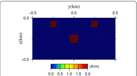
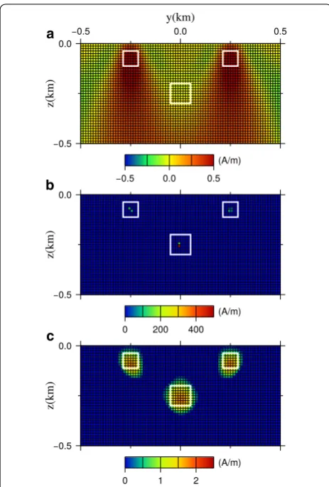
In this section, we consider a synthetic 3D magnetic model as shown in Fig. 2, which consists of three magnet-ized blocks. The model region is 1 km north-south and, 1 km east-west with depth of up to 0.5 km from the ground ( z=0 km ), and this region is divided into 80×80×40 regular grid cells. The dimensions of two shallow blocks are 75×75×75 m3 which are centered on ( − 0.25 km, 0 km, − 0.075 km), (0.25 km, 0 km, − 0.075 km), respectively, and a deep block has a dimension of 100×100×100 m3
centered on (0 km, 0 km, − 0.25 km). The perspective view of this model is displayed in Fig. 2a. The directions of the ambient geomagnetic field are assumed to be I=50◦ and D= −7◦ , and the induced magnetization of these three blocks are assumed as 2 A/m. The magnetic total field
anomaly was computed over 80×80 observation points at an altitude of 50 m above the surface. Figure 2b shows the synthetic anomaly, which is contaminated with uncor-related Gaussian noise with zero mean and a standard deviation of σ0=1.0 nT which is about 2% of the anomaly magnitude. The distribution of noise is displayed in Fig. 2c, and Fig. 3 shows a cross-section of this model through the x=0 km profile.
Using this anomaly as an input, the optimal model was obtained by L1 norm regularized inversion with CDA. The CDA is applied for a decreasing sequence in the
a
b c
Fig. 2 A synthetic model which consists three magnetized blocks.
a A perspective view of the synthetic model which displays the all non-zero model elements. The induced magnetization of each block is 2 A/m, and the directions of the ambient geomagnetic field are assumed to be I=50◦ and D= −7◦ . b The total field anomaly
computed by this synthetic model which is contaminated by an uncorrelated Gaussian noise with zero mean and a standard deviation
σ0=1.0 nT . c The histogram of the contaminated noise
range of max =103 to min=10−1 with an interval of log10(�)=0.1 on the log scale. By the L-curve method, ˆ
was estimated as 5.2 (Fig. 4).
Figure 5a shows the obtained model. In this calculation, a conventional weighting function wS1 was used. This fig-ure shows that estimated causative bodies are excessively concentrated and the actual magnetization and dimen-sions of the blocks are not well represented.
As described in the previous section, it is known that L1 norm regularization has some critical drawbacks in the case where the number of model parameters (M) greatly exceeds the number of observed data (N), which is the situation commonly seen in 3D magnetic inversion.
One major drawback is that, the number of non-zero elements of βˆ obtained by L1 norm regularization cannot exceed the number of observations N. For the theoretical explanation of this feature, please see (Tibshirani 2013) and references therein. Another major drawback of L1 norm regularization is that, if N<<M and some of the
col-umns of X are highly correlated with each other, L1 norm
regularization provides an extremely concentrated model (Fan and Li 2001). As described in the previous section, xj stores the (weighted) magnetic anomaly produced by a grid cell Vj with unit induced magnetization. Thus, as the sub-surface space is divided into very fine grid cells, the pattern of xj is similar to that of the magnetic anomaly produced by the neighborhood cells, and xj tends to be highly correlated with its neighborhood columns. As a result of these draw-backs, an overly sparse nature is promoted in the case of magnetic inversion and an excessively concentrated model is provided, as shown in Fig. 5a.
This excessively concentrated feature can be also seen in the other sparse magnetic inversion which is based on the alternative of the L0 norm regularization same as the L1 norm regularization. Actually, the result in Figure 1e of Portniaguine and Zhdanov (1999) obtained by mini-mum-support inversion is very similar with that in Fig. 5a. To avoid this problem, they used upper (and lower) lim-its for the model parameters. By introducing the bound a
b
Fig. 4 L-curve and its curvature. a An L-curve obtained by CDA for L1 norm regularized magnetic inversion. The open circles are the discrete L-curve obtained by CDA for a decreasing sequence down
from max=103 to min=10−1 with an interval of log10(�)=0.1 on the log scale. The solid line is the interpolation curve of the discrete L-curve obtained by cubic spline. b The curvature of the interpolated L-curve. The solid triangles of these figures show the point where the curvature of the interpolated L-curve takes maximum
a
b
c
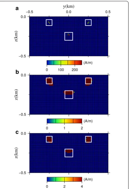
Fig. 5 Cross-sections of the synthetic model. Cross-section through the x=0 km profile of the models derived by L1 norm regularization with a no bound constraint, with bound constraint of bβ≤2 , and c
constraints, they showed that, if an appropriate bound constraint is set, the minimum-support inversion can reproduce the true model very well.
In the case of CDA, we can also introduce the bound constraint. When the upper limit βˆj≤βmax is applied, we can easily see that, because Eq. (11) is convex, βˆj(k+1) of
Eq. (16) is replaced by
and as the same manner, when lower limit βmin≤ ˆβj is applied, βˆj(k+1) is replaced by
Figure 5b shows the result of the L1 norm regulariza-tion with the bound constraint βj≤2 . From this figure, we can see that the resultant model represents the true model very well.
On the other hand, Fig. 5c shows the result with the bound constraint βj≤4 , which is twice the true value. From this figure, we can see that, the magnetization of the causative bodies was estimated larger ( ≃ 4 A/m), and the size of blocks was estimated to be smaller.
These results suggest that, in the case of the L1 norm reg-ularization with bound constraint, the value of βmax is criti-cal for the shape and magnetization of the derived model. However, when the subsurface magnetic structure of the study area is complex, it will be often difficult to choose an appropriate βmax.
Therefore, instead to set the upper limit of the model, I introduce the following combination of L1 and L2 norm penalty to reduce the overly concentrated feature of the L1 norm regularization:
where >0 is a regularization parameter, and 0≤α≤1 is a hyperparameter which represents the mixing ratio of L1 and L2 norm regularization. This modification is same as the “naive Elastic Net” proposed by Zou and Hastie (2005), and the drawbacks of the L1 norm regularization described above can be reduced theoretically as in what follows.
Obviously when α=0 , this functional becomes
and the problem of minimizing Eq. (23) is a Lagrange version of the ordinary Tikhonov regularized problem with order zero:
where
I is the M×M identity matrix, and 0 is an M -dimen-sional null column vector. So, the problem correspond-ing to Eq. (22) is a Tikhonov problem with an L1 norm constraint:
where tα is the threshold corresponding to α . Now in Eq. (25), the dimension of the “observed data” b is
N+M , which exceeds the number of unknown
param-eters M. Thus, every element of β can have a non-zero value and the first drawback of LASSO is resolved.
In addition, Zou and Hastie (2005) showed that L1–L2 norm regularization encourages a “grouping effect”, which means that the elements of the solution corresponding to the highly correlated columns of X have similar estimated values. By this enforcing of the grouping effect, the second drawback is mitigated. For the details of this point, please refer to section 2.3 of Zou and Hastie (2005).
As the result of L1–L2 norm regularization, the effect that the L1 norm regularized solution is overly concen-trated is resolved by introducing the L2 norm constraint, and at the same time, the sparse nature of the model is also provided by the L1 norm constraint.
In the next section, some synthetic tests are performed and the effectiveness of the L1–L2 norm regularization for magnetic inversion is discussed. Prior to that, the CDA algorithm and the regularization parameter selec-tion method for L1–L2 norm regularizaselec-tion are briefly described in the following subsections.
Coordinate descent algorithm for L1–L2 norm regularized problem
Then, the update equation for βˆj(k+1) is modified to
In the case of the L1–L2 norm regularized problem of Eq. (22), G(β) of Eq. (18) is
and this function is differentiable and its Hessian matrix is H =XTX+(1−α)I . In general, the product of a real matrix and its transpose XTX is positive semi-defi-nite (Cambini and Martein 2009), that is, all its eigenval-ues ej(j=1, 2,. . .,M) satisfy ej≥0 , where the number of zero eigenvalues is the dimension of the null space of X . So, when L2 norm penalty is applied together with L1 norm penalty, that is, when 0≤α <1 , the eigenvalues of H are ej+(1−α) >0 for an arbitrary >0 , and H is positive definite. Thus, G(β) of Eq. (22) is strictly con-vex for any , and it is guaranteed that CDA provides the optimal solution of Eq. (25) according to Tseng (2001).
Regularization parameter selection for L1–L2 norm regularized problem
In Eq. (22), we have to specify and α for the inversion. Friedman et al. (2010) showed the calculation results of linear regression problems using several small data sets for various with fixed α . While they suggested that an optimal can be selected by using the cross-validation method, this method is too costly for a large-scale prob-lem such as the magnetic inversion. Therefore, in this paper, the L-curve method is used to select an optimal after giving α a priori. The L-curve is plotted for the L2 residual norm versus the penalty:
The ˆ is selected as where the curvature of this L-curve reaches a maximum. However, in this procedure, there remains a problem of what value should be given to α . This point is discussed in the next section.
Synthetic examples
Synthetic test based on 3 blocks model
In this subsection, synthetic tests are performed using the proposed inversion method with L1–L2 norm
∂L(β,,α) ∂βj = −x
T
j {f −X(β−j+ejβj)} +(1−α)βj
+αsign(βj)=0.
(26) ˆ
βj(k+1)= 1
xT
j xj+(1−α)
SxT
j rˆ
(k)
−j,α
.
G(β)= 1
2||y−Xβ|| 2+ 1
2(1−α)||β|| 2,
P(β;,α)=(1−α)1
2||β|| 2
+α M
i=1 |βi|.
combined regularization. Through these synthetic tests, an appropriate value of α is discussed as well as the suit-able weighting function.
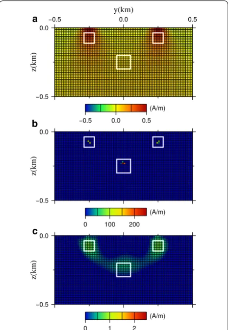
Figure 6 shows a cross-section on the x=0 km pro-file of the models obtained by the proposed inversion method using Fig. 2b as input data. In this calculation, a conventional weighting function wS1 of Eq. (9) was used. The value of α is fixed to (a) 0.0, (b) 1.0, and (c) 0.8, respectively, and the Fig. 8b is the same as that in Fig. 5a. The CDA was performed for a sequence decreas-ing from max=103 to min=10−1 with an interval of log10(�)=0.1 on the log scale. Using the L-curve method, ˆ were estimated as (a) 17.3, (b) 5.2, and (c) 3.2, respectively.
The model in Fig. 6a with α=0.0 is the result of the conventional Tikhonov regularization. In this model, while there are high-magnetization regions correspond-ing to the two shallow blocks of the true model, they are
a
b
c
Fig. 6 Optimal models derived by L1–L2 norm combined regularization. Optimal models derived by L1–L2 norm combined regularization using weighting function wS1
with aα=0.0 , and b
strongly blurred, and their shape is different from that of the true model. Further, there is no distinct high-mag-netization region corresponding to a deep block. The estimated magnetization of the resultant model is also different from that of the true model and is estimated to be smaller. Because the model of Fig. 6a has blurred fea-tures, the volume of the magnetized regions is estimated to be larger, and the magnetization is conversely esti-mated to be small.
On the other hand, the model in Fig. 6b with α=1 , which is an L1 norm regularized case, shows excessively concentrated feature as described in the previous section. While the magnetized region corresponding to the deep block can be recognized, their shape and magnetizations are completely different from that of the true model and failed to reproduce the true model.
Conversely, the model in Fig. 6c with α=0.8 is closer to the true model, and location, magnetization, and shape of the resultant model are comparable to that of the true model. From these results, we can see that, L1–L2 norm regularization with wS1 improves the reconstructivity of the model when an appropriate α is selected.
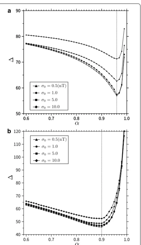
Next, to obtain an optimal α , L1–L2 norm regularized inversion was performed again while varying the value of α , and the following residual norm was calculated for each derived model:
where βˆα is the optimal model with the hyperparameter
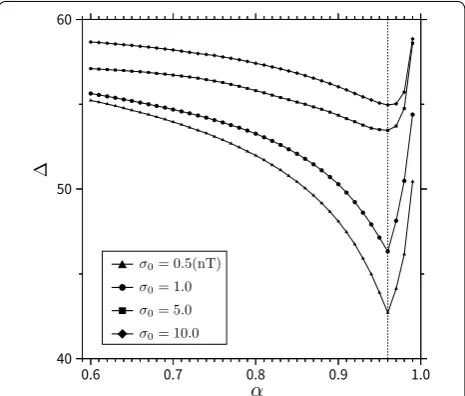
α , and βtrue is the true model shown in Fig. 2. It can be considered that, the αˆ which minimizes is an optimum α which derives the closest model to the true model in terms of the model residuals. However, it is possible that the value of αˆ changes with the amplitude of the noise. Thus, was also calculated with changing σ0 as 0.5, 1.0, 5.0, and 10 nT, respectively.
Figure 7 shows the plot of for α in the range of 0.6 to 0.99 with an interval of 0.01. In this figure, solid tri-angles, circles, squares, and diamonds indicate the case of σ0=0.5 , 1.0, 5.0, and 10.0 nT, respectively. From this figure, we can observe that, αˆS1 , that is, the optimum α in which takes minimum when wS1 is used, takes the value around 0.96 regardless of the value of σ0 . Figure 8 shows the optimal model derived with αˆS1 =0.96 using
wS1 . The ˆ was estimated as 3.07 by the L-curve method. In this figure, panel (a) shows the perspective view of the model, and (b) and (c) show the recovered anomaly and the histogram of the residuals, respectively. The standard deviations of the residuals are 0.98 nT, and this value is comparable to the true standard deviation of σ0=1.0 nT.
Next, I tried wS2 of Eq. (10) as the weighting function. Figure 9 shows the results with (a) α=0.0 , (b) α=1.0 , and (c) α=0.8 and ˆ were estimated as (a) 5.7, (b) 4.2,
�= || ˆβα−βtrue||,
and (c) 4.0, respectively. Like the model in Fig. 6a, the model of Fig. 9a is also strongly blurred, and a high-magnetization region corresponding to a deep block can not be recognized. Although high-magnetization regions corresponding to the shallow blocks can be seen,
Fig. 7 Plot of for α . Plot of for α in the range of 0.60 to 0.99 with an interval of 0.01, using the weighting function wS1
. The solid triangles, circles, squares, and diamonds indicate the case of σ0=0.5 ,
1.0, 5.0, and 10.0 nT, respectively
a
b c
Fig. 8 An optimal model derived by L1–L2 norm regularized inversion. An optimal model derived by L1–L2 norm regularized inversion with αˆS1
=0.96 using weighting function wS1
. a A perspective view of the optimum model which displays all non-zero model elements, b total field anomaly computed by this model, and
they extend to the depth direction strongly unlike the true model, and the difference from the true model is greater compared with that in Fig. 6a. This makes sense, because Li and Oldenburg (2000) pointed out wS1 is suit-able for smooth inversion. Figure 9b is the model with α=1.0 , and we can see that, the derived model is exces-sively concentrated like the model in Fig. 6b and failed to reproduce the true model. On the contrary, the model in Fig. 9c is more closer to the true model as in the case of Fig. 6c.
Figure 10 shows the plot of α versus when wS2 is used. In this figure, solid triangles, circles, squares, and dia-monds indicate the case of σ0=0.5, 1.0, 5.0 , and 10.0 nT, respectively. From this figure, we can observe that, αˆS2 , which is the optimum α when wS2 is used, takes the value around 0.90.
Figure 11 shows the result with αˆS2 =0.90 , and panels (a), (b), and (c) show the perspective view of the model,
the recovered anomaly, and the histogram of the residu-als, respectively. The standard deviations of the residuals is 1.0 nT, which is same as the true standard deviation.
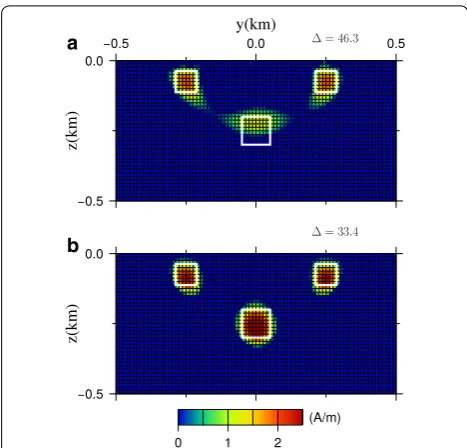
Figure 12 shows the cross-sections through the x=0 km profile of the model of (a) Fig. 8a, and (b) Fig. 11a, respectively, and the values of are also a
b
c
Fig. 9 Cross-section through the x=0 km profile. Cross-section through the x=0 km profile of the models derived by L1–L2 norm combined regularization using weighting function wS2
with a
α=0.0 , and bα=1.0.and cα=0.8 . White squares indicate the location of the magnetized blocks of the true model
Fig. 10 Plot of for α . Plot of for α in the range of 0.60–0.99
with an interval of 0.01, using the weighting function wS2
. The solid triangles, circles, squares, and diamonds indicate the case of σ0=0.5 ,
1.0, 5.0, and 10.0 nT, respectively
a
b c
Fig. 11 An optimal model derived by L1–L2 norm regularized inversion. An optimal model derived by L1–L2 norm regularized inversion with αˆS2=0.90 using weighting function wS2 . a A perspective view of the optimum model which displays all non-zero model elements, b total field anomaly computed by this model, and
displayed. From this figure, we can see that, the shape, location, and magnetization of the three magnetized blocks of the true model were reproduced well, in either case.
As described before, L1–L2 norm regularization pro-vides sparsity and smoothness in the model, and these contradictory features are provided competitively. Obvi-ously, as α decreases, the L2 norm regularization is act-ing strongly, and the resultact-ing model becomes smoother and blurred. On the contrary, when α gets close to 1, the intensity of the L1 norm regularization increases and the magnetization tends to concentrate to each center of the magnetized region. Thus, Fig. 12 suggests that, in the values around αˆS1 =0.96 , and αˆS2 =0.90 , a trade-off between the contradictory features of the L1 and L2 norm regularization is realized, and a model that is appropriately focused and is not excessively concentrated is obtained. Further, at this point, the model norm differ-ence between optimal model and true model reaches a minimum.
Next, let us focus on the performance of wS1 and wS2 . Comparing the results of Fig. 12a and b in detail, the model in Fig. 12a, which is derived by using wS1 , is slightly blurred. Especially, the depth of the deep block is esti-mated to be shallow, and magnetization is estiesti-mated to be small. From this figure, we can see that, the model in Fig. 12b is closer to the true model than that in Fig. 12a. Indeed, of the model in Fig. 12b takes a smaller value
( =33.4 ) than that of the model in Fig. 12a ( =46.3 ), which means the model in Fig. 12b is closer to the true model.
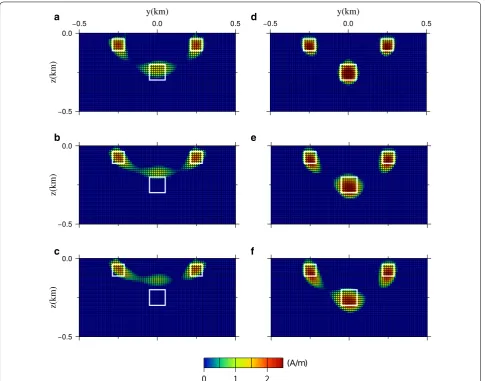
Figure 13 shows the optimal models with αˆS1 =0.96 and αˆS2 =0.90 for various σ
0 . Figure 13a–c shows the optimal models of αˆS1 =0.96 with σ
0 of (a) 0.5, (b) 5.0, and (c) 10.0 nT, and Fig. 13d–f shows the models of αˆS2 =0.90 with σ
0 of (d) 0.5, (e) 5.0, and (f) 10.0 nT, respectively. From Fig. 13a–c, we can see that, the shape of the estimated magnetized blocks becomes blurred and the depth of the deep block is estimated to be shallow as σ0 increasing. On the contrary, in the case of the models of Fig. 13d–f, depth and shape of the magnetized blocks are well reproduced, and they are comparable to the true model regardless of the noise amplitude. These results show that, by using wS2 as the weighting function, we can obtain an appropriate model robustly regardless of the noise amplitude. From these results, we can see that, wS2 seems to outperform wS1 , and wS2 is suitable for the pro-posed L1–L2 norm regularized magnetic inversion.
Synthetic test based on subducting slab model
In order to further discuss the optimal α and the per-formance of wS1 and wS2 , more synthetic tests were performed.
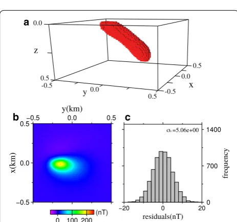
Figure 14 shows a model of subducting slab, consist-ing of 13 plates that have induced magnetization with dimension of NS 175m×EW 75m× and thickness of 25 m. The inclination of this slab is 45◦ to the depth of 2.5 km, increasing to 60◦ in the deeper part. The directions of the ambient geomagnetic field are assumed to be I =75◦ and D=25◦ , and the induced magnetization of this slab is assumed as 2 A/m.
Figure 14a shows a perspective view of this model, and Fig. 14b shows the magnetic anomaly produced by this slab which is contaminated with Gaussian noise with zero mean, and standard deviation σ0 of 5.0 nT, which is about 2% of the maximum amplitude of the anomaly. The histogram of noise is shown in Fig. 14c. Figure 15 shows a cross-section through the x=0 km profile.
Figure 16 shows the plots of for α in the range of 0.6 to 0.99 using the weighting function of (a) wS1 and (b)
wS2 . From these results, we can see that, αˆS1 and αˆS2 are about (a) 0.96 and (b) 0.90, respectively, as in the case of the three-block model of the previous subsection. This result suggests that, the values of αˆS1 and αˆS2 stably take the same values regardless of the difference in the model.
Figures 17 and 18 show the optimal models derived with αˆS1 =0.96 , and αˆS2 =0.90 , and ˆ is estimated as 16.7, and 23.1, respectively. In these figures, panel (a) shows the perspective view of the model, and (b) and c) show the recovered anomaly, and the histogram of the residuals, respectively. The standard deviations of the a
b
Fig. 12 Cross-section of the models. Cross-section of the models with aαˆS1=0.96 using weighting function wS1 , and bαˆS2=0.90
using wS2
residuals are 4.92 nT (Fig. 17c), and 5.06 nT (Fig. 18c) that are comparable to the true standard deviation of σ0=5.0 nT . Figure 19 shows the cross-sections through the x=0 km profile of the models in (a) Fig. 17, and (b) Fig. 18, respectively. The model of Fig. 19a reconstructed the shallow part of the true model. But in the deeper part, the shape of this model is different from that of the true model and failed to reproduce the slope change of the slab. On the contrary, the shape of the model in Fig. 19b is more closer to the true model, and slope change of the slab is well reproduced. Further, of the model in Fig. 19b takes a smaller value ( =46.4 ) than that of the model in Fig. 19a ( =57.4 ), that suggests the model in
Fig. 19b is closer to the true model.
From the results described in this section, it is sug-gested that, in the proposed inversion framework, that is,
L1–L2 norm combined regularized inversion with CDA, the intensity of the weights of conventional wS1 seems to be not enough in the deep part to reproduce the true model, and the weighting function wS2 seems to outper-form wS1 . By introducing the weighting wS2 , the product xT
j rˆ (k)
−j =(kjT/||kj||)rˆ (k)
−j indicates the correlation between partial residuals rˆ(k)
−j and magnetic anomaly kj . Therefore, shrinkage of the soft-thresholding operator S is per-formed with respect to the correlation between rˆ(k)
−j and
kj , and inversion becomes a correlation-based inversion.
Real data study
In this section, the proposed method was applied to aero-magnetic data observed on the northern part of Hok-kaido Island, Japan.
a d
b e
c f
Fig. 13 Optimal models derived by L1–L2 norm combined regularized inversion. Optimal models derived by L1–L2 norm combined regularized inversion with αˆS1
=0.96 and σ0 of a 0.5, b 5.0, and c 10.0 nT, with αˆS2=0.90 and σ0 of d 0.5, e 5.0, and f 10.0 nT. White squares indicate the location
On the central part of Hokkaido Island, the Kamuiko-tan tectonic belt extends from north to south for a dis-tance of about 300 km. This tectonic belt is interpreted as a Cretaceous subduction complex that formed on the old plate boundary between the Eurasian and Kula-Izanagi plates (e.g., Maruyama and Seno 1986).
Figure 20 is a simplified geological map of an area of 10 km×10 km on the northern part of Hokkaido Island, Japan. This area contains part of the Kamuikotan tec-tonic belt, which consists mainly of volcanic rocks, volcaniclastic turbidites, and sedimentary rocks. In
addition, two intrusive serpentine belts extend in the north-south direction. Within the Kamuikotan tectonic belt, serpentine blocks are intermittently seen, which is one of the characteristics of this tectonic belt.
Morijiri and Nakagawa (2005) studied the magnetic properties of the serpentine rocks that were sampled from the outcrop of the southern part of the Kamuiko-tan tectonic belt. They reported that, while these serpentine samples have large and stable remanent magnetization, their directions are randomly scattered. So, since the scattered magnetizations are canceled each other, the mean remanent magnetization of the serpentine rocks in the Kamuikotan tectonic belt is considered to be small. In the area of Fig. 20, the other a
b c
Fig. 14 A synthetic model of a subducting slab. a A perspective view of the synthetic model which displays the all non-zero model elements. The induced magnetization of each block is 2 A/m, and the directions of the ambient geomagnetic field are assumed to be
I=75◦ and D=25◦ . b The total field anomaly computed by this
synthetic model which is contaminated by an uncorrelated Gaussian noise with zero mean and a standard deviation σ0=5.0 nT. c The
histogram of the contaminated noise
Fig. 15 A cross-section of the synthetic model. A cross-section of the synthetic model of Fig. 14 through the x=0 km profile
a
b
Fig. 16 Plot of for α . Plot of for α in the range of 0.60 to 0.99 with an interval of 0.01, using the weighting function of awS1
, and bwS2
. The solid triangles, circles, squares, and diamonds indicate the case of
rocks around the serpentine belts are also expected to have small remanent magnetization because they are mainly sedimentary rocks. Thus, I assumed that the
main factor of the magnetization in this area is the induced magnetization.
On the northern part of Hokkaido Island, an aeromag-netic survey was conducted by the Geological Survey of Japan (GSJ) in 1974 for the purpose of oil and natural gas resource evaluation. These data, and other aeromag-netic data acquired by GSJ and New Energy Development Organization of Japan (NEDO) in and around Japan area, had been compiled and published as the “Aeromagnetic Anomalies Database of Japan” by the GSJ (Nakatsuka and Okuma 2005). The data on the area of Fig. 20 that contained in this database are a projection of the IGRF residuals onto a regular grid of 200 m×200 m at a uni-form altitude of 1,524 m above sea level using upward continuation.
In this paper, the shallow magnetic structure of the area of Fig. 20 was investigated by applying the proposed magnetic inversion method. The study area was divided into 50×50×35 regular grid cells up to a depth of 3.5 km from the surface. The dimension of each grid cell is 200×200×100 m3 , and its horizontal size is same as the spacing of the data points.
Before performing the inversion, the regional component was removed by applying trend surface analysis (Borcard et al. 1992). The regional anomaly t was assumed to be expressible by the following linear equations:
t=c0+c1x+c2y,
a
b c
Fig. 17 An optimal model derived by L1–L2 norm regularized inversion. An optimal model derived by L1–L2 norm regularized inversion with αˆS1=0.96 using weighting function wS1 . a A
perspective view of the optimum model which displays all non-zero model elements, b total field anomaly computed by this model, and
c histogram of the residuals
a
b c
Fig. 18 An optimal model derived by L1–L2 norm regularized inversion. An optimal model derived by L1–L2 norm regularized inversion with αˆS2
=0.90 using weighting function wS2
. a A perspective view of the optimum model which displays all non-zero model elements, b total field anomaly computed by this model, and
c histogram of the residuals
a
b
Fig. 19 Cross-section of the models. Cross-section of the models with aαˆS1=0.96 using weighting function wS1 , and bαˆS2=0.90
using wS2
. White line indicates the location of the magnetized slab of the true model. On the upper right of each panel, the value of is
where x and y are the coordinates of the observation points. The coefficients c0 , c1 , and c2 were estimated by least-squares fitting. Figure 21a shows the trend removed anomaly by subtracting t from the data of our study area. These data were used as the input data of our inversion.
According to Ueda et al. (2012), the magnetic incli-nation, decliincli-nation, and intensity of the total field are
assumed to be I =59.1◦ , D=N10.6◦W , and 51,000 nT, respectively.
The L1–L2 norm regularized inversion with α=0.9 was applied for a decreasing sequence down from max=103 to min=10−1 with an interval of log10(�)=0.1.
Figure 22 shows the L-curve and its curvature, and from this result, ˆ is estimated as 31.6. Figure 23 shows Fig. 20 A simplified geological map of the northern part of Hokkaido Island, Japan. A simplified geological map of the northern part of Hokkaido Island, Japan (Original map is Seamless Digital Geological Map of Japan of GSI: https ://gbank .gsj.jp/seaml ess). The left and lower coordinates of these maps are WGS84 (degree), and right and top coordinates are UTM (km)
a b
the slice of the optimal model, and recovered anomaly by this model is shown in Fig. 21b. The depth of each slice of Fig. 23 is (a) 200 m, (b) 400 m, (c) 600 m, and (d) 800 m, respectively. On each figure, the location of the exposed serpentine belts is displayed in black solid lines. As shown in this figure, a focused model was obtained exhibiting two high-magnetization areas extending north to south.
From Fig. 23a, we can see that, these two magnetiza-tion areas correspond well to the locamagnetiza-tions where two serpentine belts are exposed on the surface, and this suggests that the estimation of the subsurface magnetic structure has been successfully conducted.
Next, focusing on the magnetization intensity, the estimated magnetization of this area has a maximum of about 10 A/m. In this area, Okazaki et al. (2011) meas-ured the susceptibility of major rock samples near the surface and reported that the average susceptibility of the serpentine belt is 20×10−3 SI unit. Thus, if geomagnetic intensity is 51,000 nT, the induced magnetization is about 1 A/m, which is 10 times smaller than the estimated
value. Therefore, it can be considered that the magnetic susceptibility of the sample near the ground surface was weakened by weathering. Or, while the rock magneti-zation of this area was assumed to be only the induced magnetization, it is thought that the component of the remanent magnetization is also included.
Discussion
In this paper, a magnetic inversion combining L1 and L2 norm regularization was proposed. However, it is also possible to consider some variants of the pen-alty. For example, instead of the L2 solution norm, first-order or second-order differential solution norms could be used. By using these penalties combined with the L1 norm penalty, the problem is equivalent to a first-order or second-order Tikhonov problem with an L1 norm constraint. By introducing a differential norm penalty, the resultant model will have a smoother nature and tends to be more blurred. However, Fedi et al. (2005) suggest that higher order Tikhonov regu-larization has higher depth resolution than zero-order Tikhonov regularization in some situations. The eval-uation of the properties and validity of these penalty combinations for magnetic inversion is left as work for the future.
In this paper, methods of regularization parameter selection were also proposed that are based on the L-curve criteria. However, it will be possible to use other regularization parameter selection criteria. For example, one of the major competitors of the L-curve is generalized cross-validation (GCV) (Wahba 1990). GCV is also widely used for parameter selection in both L1 and L2 norm regularized problems. While Hansen and O’leary (1993) claimed that the L-curve outperforms the GCV for the Tikhonov problem, other studies show GCV can select feasible regulari-zation parameters (e.g., Farquharson and Oldenburg 2004). This discrepancy arises from the different con-ditions in each problem, such as the difference of the dimensions of the problem, the degree of ill-posed-ness and the noise level. The estimation of the effec-tiveness of other criteria will also considered in future work.
Conclusions
In this paper, an inversion method to obtain a 3D mag-netic susceptibility distribution has been presented which incorporates a sparseness constraint based on L1 norm regularization. In order to improve the depth resolution of the model, an appropriate weighting func-tion for the L1 norm regularized magnetic inversion has been discussed by synthetic data tests, and it is shown that the proposed square of the sensitivity weighting a
b
Fig. 22 a An L-curve obtained by CDA for L1–L2 norm regularized magnetic inversion. The open circles are the discrete L-curve obtained by CDA for a decreasing sequence down from max
=103
to min
=10−1 with an interval of log
function outperforms other competitors. However, by applying L1 norm regularization solely, the synthetic test revealed that an excessively concentrated model is likely to be obtained regardless of the dimensions of the true model. To address this problem, a combination of L1–L2 norm regularization has been introduced in this paper. To choose feasible regularization parameters of the L1 and L2 norm penalty, this paper proposed regulariza-tion parameter selecregulariza-tion methods based on the L-curve method with fixing the mixing ratio of L1 and L2 norm regularization. The synthetic tests and a real data study showed the effectiveness of the proposed inversion method.
Abbreviations
LASSO: Least absolute shrinkage and selection operator; CDA: Coordinate descent algorithm; GSJ: Geological survey of Japan; NEDO: New energy devel-opment organization of Japan; GCV: Generalized cross-validation.
Acknowlegements
The author thanks Paul Wessel and the University of Hawaii for providing Generic Mapping Tools software (https ://www.soest .hawai i.edu/gmt). Maps and graphs in this paper were drawn using this great tool. The author also would like to thank the editor and two reviewers for their valuable comments and suggestions to improve the quality of the paper.
Authors’ contributions
This manuscript has one author. The author performed the whole part of this study. The author read and approved the final manuscript.
Funding
This work is supported by JSPS (Japan Society for the Promotion of Science) KAKENHI Grant-in-Aid for Scientific Research (C), Grant Numbers JP26350475, and JP19K04967.
a
b d
c
Availability of data and materials
Not applicable.
Competing interests
The author declare that they have no competing interests.
Received: 1 April 2019 Accepted: 19 June 2019
References
Abedi M, Siahkoohi H, Gholami A, Norouzi G (2015) 3d inversion of magnetic data through wavelet based regularization method. Int J Min and Geo-Eng 49:1–18. https ://doi.org/10.22059 /ijmge .2015.54360
Bhattacharyya BK (1964) Magnetic anomalies due to prism-shaped bodies with arbitrary polarization. Geophysics 29:517–531
Borcard D, Legendre P, Drapeau P (1992) Partialling out the spatial com-ponent of ecological variation. Ecology 73:1045–1055. https ://doi. org/10.2307/19401 79
Cambini A, Martein L (2009) Generalized convexity and optimization, theory and applications. Springer, Berlin. https ://doi.org/10.1007/978-3-540-70876 -6
Fan J, Li R (2001) Variable selection via nonconcave penalized likelihood and its oracle properties. J Am Stat Assoc 96:1348–1360. https ://doi. org/10.1198/01621 45017 53382 273
Fang H, Zhang H (2014) Wavelet-based double-difference seismic tomogra-phy with sparsity regularization. Geotomogra-phys J Int 199:944–955
Farquharson CG, Oldenburg DW (2004) A comparison of automatic techniques for estimating the regularization parameter in non-linear inverse problems. Geophys J Int 156:411–425
Fedi M, Hansen PC, Paoletti V (2005) Analysis of depth resolution in potential-field inversion. Geophysics 70:1–11. https ://doi. org/10.1190/1.21224 08
Friedman J, Hastie T, Hofling H, Tibshirani R (2007) Pathwise coordinate optimi-zation. Ann Appl Stat 1:302–332. https ://doi.org/10.1214/07-AOAS1 31 Friedman J, Hastie T, Tibshirani R (2010) Regularization paths for generalized
linear models via coordinate descent. J Stat Soft 33:1–22
Hansen PC (2001) In: Johnstion P (ed) The L-curve and its use in the numerical treatment of inverse problems. WIT Press, Southamptopn
Hansen PC (1992) Analysis of discrete ill-posed problems by means of the l-curve. SIAM Rev 34:561–580
Hansen PC, O’leary DP (1993) The use of the l-curve in the regularization of discrete ill-posed problems. J Sci Comput 6:1487–1503
Honsho C, Ura T, Tamaki K (2012) The inversion of deep-sea magnetic anoma-lies using akaike’s bayesian information criterion. J G R 117(B1). https :// doi.org/10.1029/2011J B0086 11
Last BJ, Kubik K (1983) Compact gravity inversion. Geophysics 48:713–721 Li Y, Oldenburg DW (1996) 3-d inversion of magnetic data. Geophysics
61:394–408
Li Y, Oldenburg DW (2000) Joint inversion of surface and three-component borehole magnetic data. Geophysics 65:540–552
Liu G, Song C, Lu Q, Liu Y, Feng X, Gao Y (2015) Impedance inversion based on l1 norm regularization. J Appl Geophys 120:7–13
Loris I, Nolet G, Daubechies I, Dahlen FA (2007) Tomographic inversion using l1-norm regularization of wavelet coefficients. Geophys J Int 170:359–370 Maruyama S, Seno T (1986) Orogeny and relative plate motions, example of
the Japanese islands. Tectonophysics 127:305–329
Minami T, Utsugi M, Utada H, Kagiyama T, Inoue H (2018) Temporal variation in the resistivity structure of the first nakadake crater, aso volcano, Japan, during the magmatic eruptions from november 2014 to May 2015, as inferred by the active electromagnetic monitoring system. Earth Planets Space 70(1):138. https ://doi.org/10.1186/s4062 3-018-0909-2
Morijiri R, Nakagawa M (2005) Small-scale melange fabric between serpent-inite block and matrix magnetic evidence from the mitsuishi ultramafic rock body, Hokkaido, Japan. Tectonophysics 398:33–44
Nakatsuka T, Okuma S (2005) Aeromagnetic anomalies database of Japan. Dig Geosci Map P-6. Geol Surv Japan
Ogawa Y, Uchida T (1996) A two-dimensional magnetotelluric inversion assuming gaussian static shift. Geophys J Int 126(1):69–76. https ://doi. org/10.1111/j.1365-246X.1996.tb052 67.x
Okazaki K, Mogi T, Utsugi M, Ito Y, Kunishima H, Yamazaki T, Takahashi Y, Hashimoto T, Ymamaya Y, Ito H, Kaieda H, Tsukuda K, Yuuki Y, Jomori A (2011) Airborne electromagnetic and magnetic surveys for long tunnel construction design. Phys Chem Earth 36:1237–1246
Pilkington M (1997) 3-d magnetic imaging using conjugate gradients. Geo-physics 62:1132–1142
Pilkington M (2009) 3d magnetic data-space inversion with sparseness con-straints. Geophysics 74:7–15
Portniaguine O, Zhdanov MS (1999) Focusing geophysical inversion images. Geophysics 64:874–887
Portniaguine O, Zhdanov MS (2002) 3-d magnetic inversion with data com-pression and image focusing. Geophysics 67:1532–1541
Rezaie M, Moradzadeh A, Nejati KA (2016) 3d gravity data-space inversion with sparseness and bound constraints. J Min Environ 14:1–9. https ://doi. org/10.22044 /jme.2015.558
Sacchi MD, Ulrych TJ (1995) High resolution velocity gathers and offset space reconstruction. Geophysics 60:1169–1177
Tibshirani RJ (1996) Regression shrinkage and selection via the lasso. J R Statist Soc B 58:267–288
Tibshirani RJ (2013) The lasso problem and uniqueness. Electron J Stat 7:1456–1490. https ://doi.org/10.1214/13-EJS81 5
Tikhonov AN, Arsenin VY (1977) Solution of Ill-posed problems. Wiley, New York
Tseng P (2001) Convergence of a block coordinate descent method for non-differentiable minimization. J Opt Theory Appl 109:475–494
Tsunakawa H, Shibuya H, Takahashi F, Shimizu H, Matsushima M, Matsuoka A, Nakazawa S, Otake H, Iijima Y (2010) Lunar magnetic field observation and initial global mapping of lunar magnetic anomalies by map-lmag onboard selene (kaguya). Sp Sci Rev 154(1):219–251. https ://doi. org/10.1007/s1121 4-010-9652-0
Ueda I, Abe S, Goto K, Ebina Y, Ishikura N, Tanoue S (2012) Geomagnetic charts for the epoch 2010.0. J Geospat Info Auth Jpn 123:9–19 in japanese Uieda L, Barbosa VCF (2012) Robust 3d gravity gradient inversion by planting
anomalous densities. Geophysics 77:55–66
Wahba G (1990) Spline models for observational data. SIAM, Philadelphia, PA Wang Y (2011) Seismic impedance inversion using l1-norm regularization and
gradient descent methods. J Inv Ill-posed problems 18:823–838 Wang J, Meng X, Li F (2015) A computationally efficient scheme for the
inver-sion of large-scale potential field data, application to synthetic and real data. Comput Geosci 85:102–111
Xiang Y, Yu P, Zhang L, Feng S, Utada H (2017) Regularized magnetotelluric inversion based on a minimum-support gradient stabilizing functional. Earth Planets Space 69(1):158. https ://doi.org/10.1186/s4062 3-017-0743-y Zeyen H, Pous J (1991) A new 3-d inversion algorithm for magnetic total field
anomalies. Geophys J Int 104(3):583–591. https ://doi.org/10.1111/j.1365-246X.1991.tb057 03.x
Zhang L, Koyama T, Utada H, Yu P, Wang J (2015) A regularized three-dimen-sional magnetotelluric inversion with a minimum gradient support constraint. Geophys J Int 189:296–316
Zhdanov MS, Fang S, Hursan G (2000) Electromagnetic inversion using quasi-linear approximation. Geophysics 65:1501–1513
Zhdanov MS, Dmitriev VI, Fang S, Hursan G (2000) Quasi-analytical approxima-tions and series in electromagnetic modeling. Geophysics 65:1746–1757 Zhdanov MS, Ellis R, Mukherjee S (2004) Three-dimensional regularized
focus-ing inversion of gravity gradient tensor component data. Geophysics 69:925–937
Zou H, Hastie T (2005) Regularization and variable selection via the elastic net. J R Stat Soc B 67:301–320
Publisher’s Note