MODELING AND SIMULATION OF GRID CONNECTED PHOTOVOLTAIC DISTRIBUTED GENERATION SYSTEM

(1)

ISSN: 1992-8645 www.jatit.org E-ISSN: 1817-3195

448

NUMERICAL ANALYSIS OF THERMAL ENVIRONMENT IN

A NATURAL VENTILATION SUNLIGHT GREENHOUSE

1

ZHENYU DU, 2 LEI JIA, 1 DIDI XUE

1_{College of Environment Science and Engineering, Taiyuan University of Technology, Taiyuan, China} 2_{Sino-Coal International Engineering Group Nanjing Design and Research Institute, Nanjing, China}

ABSTRACT

This paper using the corresponding test data gained from the continuous environmental test in a natural ventilation sunlight greenhouse in Taiyuan, established a mathematical model of the thermal environment in such a greenhouse based on the conservation laws of mass, momentum and energy. The complex boundary conditions in CFD simulation of a sunlight greenhouse was dealt preferably with this new model. According to the unsteady simulation of the distribution and change of the temperature field in natural ventilation sunlight greenhouse based on the new model, simulation result highly matches up to the locale test data under the unsteady condition, and this model can be used to predict the thermal environment of such a greenhouse and optimize the prediction.

Keywords: Sunlight Greenhouse, Natural Ventilation, Thermal Environment, Numerical Simulation， Computational Fluid Dynamics

1 INTRODUCTION

CFD simulation can not only simulate the heat and mass transfer process inside and outside of the sunlight greenhouse, but also can provide some information of the environment in sunlight greenhouse. This will reduce the cost of experiment. In recent years, the application of the sunlight greenhouse is in the ascendant. A mathematic model of micro climate has been built in 1994[1]. Unsteady simulation of the heat condition and temperature field was conducted in greenhouse which is located in the northeast of china in 2005[2]. In the foreign countries, from 1989, CFD simulation was used to study the situation of ventilation in Venlo greenhouse without crop in the first time[3], literature [4-6]used CFD to study various kinds of greenhouses in the field of natural ventilation and heat or humidity problem with unsteady simulation. The paper of scholar in foreign countries rarely involved sunlight greenhouse because the sunlight greenhouse is produced by Chinese and the intellect property is at Chinese own. In this paper, the method to deal with boundary conditions in CFD simulation of natural ventilation is based on the experiment which is related to the heat and humidity in sunlight greenhouse in Taiyuan. Three dimensional CFD

model of natural ventilation is built and be checked by the data in experiment.

2 BUILDING MODELS 2.1. GEOMETRY MODELS

(2)

449

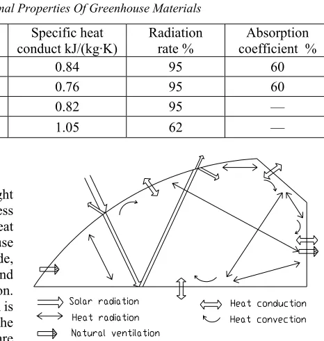
Table 1: Parameters Of Thermal Properties Of Greenhouse Materials

Material Density _kg/m Heat conduct rate _W/(m·K) _{conduct kJ/(kg·K)}Specific heat Radiation _{rate %} _{coefficient %}Absorption

brick 1650 0.62 0.84 95 60

Tile 600 0.15 0.76 95 60

Quilt 400 0.08 0.82 95 —

PVC film 1360 0.15 1.05 62 —

2.2 Thermal Physical Models

The process of natural ventilation in sunlight greenhouse is very complicated. This process include many phenomena such as fluent of air, heat convection, heat conduction in soil and greenhouse enclosure, solar radiation, thermal radiation inside, evaporation and condense of vapor from soil and plants, the concentration balance of CO2 and so on. The focal point of simulation in natural ventilation is the change of temperature and energy transmit by the fluent of air inside. The following assumptions are based on prior knowledge and the important environmental influencing factors:greenhouse materials has the same temperature and character in every direction;heat storage of the greenhouse materials are ignored; absorption rate of every solid wall towards radiation is constant; the wall that participate in thermal radiation is aimless gray surface; the influence of plants inside are ignored because they were so small in the time of young seedling. The thermal physical model is in Fig. 2 based on these assumptions.

[image:2.612.290.523.93.338.2]

Figure 1: Profile Picture Of Experimental Sunlight Greenhouse

Figure 2: The Thermal Physical Model Of Sunlight Greenhouse

2.3 Mathematic Models

2.3.1 Governing Equation Of Cfd

In the process of natural ventilation, it has not only the convection between the air inside and outside, but also the natural convection by buoyancy. The assumption of Boussineqs is used to deal with buoyancy lift which comes from the range of temperature; densities are all constant except one which is related to volumetric force in momentum equation. Governing equations are suitable for natural heat convection above as follows [7]：

( )

,

( eff )

t div V grad S

ρφ

φ φ

ρ φ φ

∂

∂ + − Γ =

r

[image:2.612.89.524.480.740.2]

(1) Sφ =SN+SB (2) Where Φ,Γφ,eff,SNand SBare in the table2.

Table 2: Φ,Γ_φ_,_eff ,S_Nand S_B

Φ Γφ,eff SN SB

1 0 0 0

i

V µeff

( j)

eff i

i j V

x P

x x

µ ∂

∂ ∂ ∂

− +

∂ ∂

θ β

ρ i

P g C

(3)

450

ε µ σeff ε ε(c G c1 − 2ρε) /k C3_KGB

ε

H µeff σH SH 0

( i j) i

t

j i j

V

V V

G

x x x

µ ∂ ∂ ∂

= +

∂ ∂ ∂ ,

t B i

P H i

G g

C x

ν

β θ

ρ

σ ∂ =

∂

In the table c1,c2 ,c3 ,cD are coefficients of k—εmodel of turbulence；σK, σε,σHare value of Schmidt or Prandtl；µeffis coefficient of effective stickiness；Vjis component of velocity；K is kinetic energy in turbulence；εis loss rate of kineticenergy in turbulence；H=cpT，is the enthalpy；µtis the coefficient of stickiness in turbulence；νt is the coefficient of stickiness in turbulence energy；gi is component of gravity；cpis specific heat at constant pressure；ϕ is current variable；β is coefficient of expand in volume；θ=H H− 0is relative enthalpy，

0

H is the value of reference ；

1

c ,c2,c3,cD,σK,σεand σH are in the literature [7]。

2.3.2 Spreading equation of solar radiation When the ray goes forward in the translucent materials, the incident ray in it is repeated reflection, absorption and transmission between two surfaces, so the total reflection rate, absorption rate and the transmission rate are the sum of each infinite item of the sun in the film layer repeatedly reflected, absorption and transmission.

The absorption rate is:

(

)

(

)

₂

(

)

2

1 1 1 1

a r r a r a

α₌ ₋ ⎡ ₊ ₋ ₊ ₋ ₊ ⎤

⎣ LL⎦

(

)

(

)

1

1 1

a r

r a

− =

− −

(3)

The reflection rate is:

(

) (

2

)

2

{

(

)

2 2

}

1 1 1 1 1

r a r a r

ρ= ⎡ + − − + − + ⎤

⎣ LL⎦

(

) (

)

(

)

2 2

1 1

1

1 1

a r

r

r a

⎡ ₋ ₋ ⎤

= ⎢ + ⎥

− −

⎢ ⎥

⎣ ⎦

(4)

The transmission rate is：

(

₁ _a

)(

₁ _r

)

2 ₁ _r2

(

₁ _a

)

2

τ= − − ⎡_⎣ + − +_LL⎤_⎦

(

) (

)

(

)

2

2 2

1 1

r a

− −

=

− − (5)

Where r is the ratio of the ray which was reflected in interfaces of the two medium; a is the ratio of the ray which was absorbed though the film layer.

The light transmittance of the greenhouse directly affects the intensity of illumination, and it is affected by the greenhouse’s location, type, structure, the arrangement of the equipment, type and the degree of aging of the transparent material, condensation of moisture and pollution degree of the translucent covering material and other factors. The light transmittance of the greenhouse can be calculated by the following equation:

D D d d

I=I τ +Iτ (6)

Where I is the strength of illumination in the greenhouse, W/m2_;

D

I is the direct solar radiation intensity arrives to the outdoor wall of the greenhouse, W/m2 _;

d

I is the diffuse solar radiation intensity arrives to the outdoor wall of the greenhouse, W/m2 _;

D

τ ,τ_dare the transmittance of direct and diffuse light of the thin film.

Regarding medium with the properties of absorption, launch and diffuse, in the positionrv, along the directionsv, the radiation transfer equation (RTE) is:

4 ₄

2

0

( , )

( ) ( , )

( , ) ( , ) 4

s

s dI r s

I r s ds

T

n πI r s s s d

α σ

σ σ α

π π

+ +

′ ′

= +

∫

Φ Ω

v v

v v v v

(7)

(4)

451 faction; Ω′ is solid angle in space, (α σ+ _s)s is the medium optical depth.

Various kinds of computation models have its characteristic and applicable scope, to some certain questions, some radiation model is possible more suitable than others. Therefore, all factors should taken into consideration such as optical depth, diffuse and launch, gas and particle radiation heat transfer, translucent medium and mirror surface boundary, partial heat source and so on when determinate using what radiation models. In this paper, greenhouse's optical depth is smaller than 1, and it has the translucent medium (the PVC membrane), besides, the whole space is not completely closed due to the supply-air outlet and exhaust outlet. Discrete model can simulate the process of radiation in Translucent Materials; it has been chosen to calculate the influent to temperature inside the greenhouse from solar radiation. This model regards the radiation transfer equation (RTE) disseminated along x direction as some field equations. Thus, the equation (7) changes into:

4 ₄

2

0

( ( , ) ) ( ) ( , )

( , ) ( , ) 4

s

I r s s I r s

T

n πI r s s s d

α σ σ σ α

π π

∇ ⋅ + +

′ ′

= +

_∫

Φ Ω

v v v v v

v v v v

(8)

What separate Coordinate model (DO) solves is radiation transfer equation (RTE) which send out by the limited solid angle, and each solid angle is corresponding the fixed direction sv in the coordinate system (Descartes). Solid angle separate precision was determined by the user, and it is a little similar to the ray number in the DTRM model. But the different is, the DO model does not carry on the ray tracing, on the contrary, it transforms the equation (7) to the transportation equation of radiation intensity under the three-dimensional coordinate system. Every (solid angle) direction sv

can solve a (radiation intensity) transportation equation, and the solving methods are as same as the methods to solve fluid flow and energy equation. The separate Coordinate model uses format of conservation difference which is called limited volumetric method, and this difference method expands to the non-structuring grid afterwards. 2.3.3 Unsteady equation of heat conduction [8]

The different equation of wall to describe the one dimension heat conduct T x( , )τ is as follows:

2

( , ) ( , )

T x T x

a x

τ τ

τ

∂ ₌ ∂

∂ ∂

(9) Heat conduction quantity q x( , )τ satisfies Fourier law：

( , ) ( , ) T x q x

x

τ

τ = −λ∂

∂ (10)

Where ais coefficient of heat conduct of solid materials, a

c

λ ρ

= m2_/s_；_λ_{is coefficient of heat}

conduct of wall materials，W/（m⋅K）；ρis the density of wall materials，kg/m3_； _c_{is specific}

heat conduct of wall materials, kJ/(kg⋅K).

As for the calculation to the unsteady heat transfer of the wall, Laplace transform is used to solve it. The Laplace transform of heat conduction partial differential’s equation transforms original equation into algebraic equation gradually, and then the transition matrix of the wall thermodynamic system or the s-transfer function will be obtained through the equation set after transformation, finally Laplace transform's expression according to the boundary condition will be solved. The s-transfer function relations between input and output at both sides of the wall deduced by Laplace transform are as follows:

Regarding heat absorption outside the building enclosure:

( )

(0, ) (0, ) 0

( ) r

A s

Q s T s t

B s

= =

(11) Regarding heat absorption inside the building enclosure:

( )

,

_{( ) ( )}

( )

, a 0

D s

Q l s T l s t

B s

= − =

(12)

Regarding heat transfer inside the building enclosure:

( )

, 1

_{( ) ( )}

0, r 0

Q l s T s t

B s

= =

(13) Where x l= is the thickness of the wall, m, ( , ) [ ( , )]

(5)

452 temperature outdoor, Ԩ; ( )A s、B s( )、D s( ) are the elements of matrix in s-transfer function of the wall thermodynamic system.

Boundary condition can be separated into unit harassing quantities with the same time interval and distributed according to time series if temperature of boundary condition continuous changing with time is not periodic function. And the isosceles triangular wave method is used to separate a given harassing quantity curve. In order to calculate the heat transmission conveniently, firstly, making the time discrete, namelyτ= ∆j τ . Then using the above relationships can obtain the heat absorption and heat transfer reaction factors,X j( ) Z、 ( )j and ( )Y j , of the building enclosure easily.

The heat transfer reaction coefficient of the discrete building enclosure are:

1

2 ( 1) 1

0, (0) (1 )

1, ( ) (1 )

i i i i i j i i B

j Y K e

B

j Y j e e

α τ

α τ α τ

τ τ ∞ − ∆ = ∞ − ∆ − − ∆ = = = + − ∆ ≥ = − − ∆

∑

(14) The heat absorption reaction coefficient are:

1

2 ( 1) 1

0, (0) (1 )

1, ( ) (1 )

i i i i i j i i A

j X K e

A

j X j e e

α τ

α τ α τ

τ τ ∞ − ∆ = ∞ − ∆ − − ∆ = = = + − ∆ ≥ = − − ∆

∑

(15) 1

2 ( 1) 1

0, (0) (1 )

1, ( ) (1 )

i i i i i j i i C

j Z K e

C

j Z j e e

α τ

α τ α τ

τ τ ∞ − ∆ = ∞ − ∆ − − ∆ = = = + − ∆ ≥ = − − ∆

∑

(16) The sub-matrix elements of a multi-layered wall are:

( ) ( ) ( )

i i i

i

s

A s D s ch l

a

= = (17)

( ) ( ) i i i i i s sh l a B s s a λ

= (18)

( ) ( )

i i i

i i

s s

C s sh l

a a

λ

= (19)

The north wall in the greenhouse using response coefficient method to calculate the heat transfer, thermal physical parameters of the north wall material are shown in Table 1. The formula (14) ~ (19) are using computer programming to calculate the reaction coefficient of the wall, and the results are shown in table 3.

Table3: The Reaction Coefficient Of Wall

J X(J) Y(J) Z(J)

0 51.14104 6.736245 93.43117 1 -50.13063 -5.873682 -92.26373 2 -0.301637 -0.1592826 -0.3517753 3 -3.74E-02 -0.0303096 -8.25E-02 4 -1.00E-02 -1.02E-02 -3.30E-02 5 -3.82E-03 -4.46E-03 -1.65E-02 6 -1.79E-03 -2.26E-03 -9.46E-03 7 -9.69E-04 -1.27E-03 -5.91E-03 8 -5.79E-04 -7.71E-04 -3.93E-03 9 -3.74E-04 -4.89E-04 -2.74E-03 10 -2.55E-04 -3.19E-04 -1.99E-03 11 -1.83E-04 -2.10E-04 -1.48E-03 12 -1.35E-04 -1.37E-04 -1.13E-03 13 -1.02E-04 -8.74E-05 -8.82E-04 14 -7.94E-05 -5.37E-05 -6.99E-04 15 -6.26E-05 -3.14E-05 -5.63E-04 16 -5.01E-05 -1.73E-05 -4.60E-04 17 -4.06E-05 -8.94E-06 -3.80E-04 18 -3.33E-05 -4.73E-06 -3.17E-04 19 -2.76E-05 -3.29E-06 -2.67E-04 20 -2.32E-05 -3.65E-06 -2.27E-04 21 -1.97E-05 -5.08E-06 -1.94E-04 The quantity of heat transfer in wall at the time m can be calculate by the methods of response factor with boundary condition that air temperature in two sides changes along with time.

0 0

( ) ( ) (_z ) ( ) (_r )

j j

HG m ∞ Y j t m j ∞ Z j t m j

= =

=

∑

− +

∑

−

(6)

453 3 SOLVE E QUATIONS

3.1 Meshing

[image:6.612.90.301.252.459.2]

A closed region inside the greenhouse that has a length of 9.2m was chosen to be calculated. The unstructured grid is used to divide irregular regions, the meshes are divided and calculated again and again in the region that has notable change grad d at the entrance of fluent. Meshes which are excellent in uniformity will be chosen after checking them. There are 34468 nodes，163993 volume grids, as shown in Fig. 3.

Figure 3: Grid plotting of greenhouse

3.2 Solving And Disserting Of Equations

Discrete forms, methods and settings of solving are in the table 4.

Table 4: Preferences Setting Of Solving

Solver Turbulence _model Radiation model Couple of pressure _{and velocity} relaxation Under factor

Separated k-ε model DO model PISO 0.3～1.0

Pressure

disperse form disperse form Energy disperse form Density disperse form Momentum k disperse form ε disperse form Body force

weighted Second order upwind Second order upwind Second order upwind First order upwind First order upwind

3.3 Confirm The Condition Of Solving 3.3.1 Initial condition

The data in experiment used to test and verify the result from unsteady simulation is picked up from one day 8:00am to 16:00pm. The initial value of temperature is the data that test from experiment at the initial moment, the initial value of velocity is the

data that test from steady simulation at the initial moment.

3.3.2 Boundary condition

[image:6.612.83.530.515.636.2]

(7)

454 to deal with solar radiation. Outside comprehensive temperature, inside temperature, respond coefficient and heat flux through the wall all are in the literature [9]. The settings of other boundary conditions are as follows:

（1）the setting of temperature in entrance, film and soil

Based on the data in experiment, mathematic statistics is used to build the un-linear one dimensional equation to describe T₁ (temperature in entrance), T2 (temperature of film), T3 (soil

temperature):

13 3 8 2 5

1( ) 5.37 10 2.21 10 3.12 10 284.6

T t _{= −} _× − t ₊ _× −t ₊ _× −t₊

(20)

12 3 8 2 4

2( ) 3.20 10 8.10 10 7.16 10 290.4

T t _{= −} _× − t ₊ _× −t ₊ _× −t₊

(21)

12 3 8 2 4

3( ) 1.93 10 5.30 10 2.62 10 290.5

T t _{= −} _× − t ₊ _× −t ₊ _× −t₊

(22) Coefficient of dependence of the above three equations is 0.9792、0.9617、0.9641; it makes clear that above temperatures are related to the flow time, so the equations above can give the law of temperature changing with time.

（2）the setting of wall

Based on the quantity of heat flux in translucent wall from 8:00am to 16:00pm which is calculated by the method of respond coefficient, mathematic statistics is used to build the un-linear one dimensional equation to describe the Q (quantity of heat flux) and t(flow time ):

12 3 8 2 4

( ) 1.21 10 7.9 10 1.35 10 14.406

Q t ₌ _× − t ₋ _× −t ₊ _× −t₊ ₍₂₃₎

Coefficient of dependence is 0.9893，it makes clear that above temperature is related to the flow time and the equations can give the law of changing in heat flux .

Express the above four regression equations with the C language source code, and then establish a C language source code file, translate the UDF function and connects FLUENT, carry out UDF in FLUENT to calculate it.

[image:7.612.316.510.547.677.2]

4 RESULT OF UNSTEADY SIMULATION Fig. 4 is the inside temperature change of the maxim and minimum value. It can be found that the maxim value, minimum value and the distance them

all changed with flow time, and the laws of their changes are similar. It can explain that the inside temperature depends on outside obviously. Solar radiation gives the biggest effect to maxim value of inside temperature at 13:30; and the minimum value inside is in the entrance, it reached its top at14:30; the above law can be concluded that inside temperature mainly depends on the solar radiation outside but the temperature outside.

Fig. 5 gives the result of temperature field of three different profiles in different time. From it, it is obviously that the region which is nearly by plastic film changes in the biggest extent; the phenomena can be another reason to conclude that inside temperature mainly depends on the solar radiation outside.

Comparing the temperature distribution of each time, it is known that the temperature distribution has a little different in each height at different time, but the tendencies are almost the same; a little more obvious law appeared at 16:00，the maxim value appeared near the film, and the range of change in height is more obvious than length. The data from simulation and experiment have the similar distribution and the change tendency.

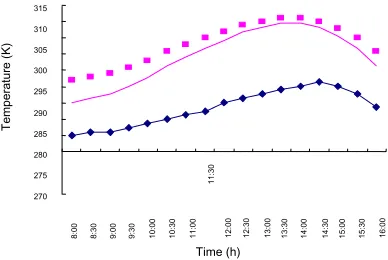
Fig. 6 is the compare of experiments and calculates at 9:00. The maxim distance of them is 4.9K which appears at the edge near by the rooftop; the minimum distance is only 3.5K in the whole region; the maxim distance of experiment and calculate is less than 4.5K except the edge. Although there are some different between experiments and calculates, the law of them are similar. All of these prove that the three dimensional unsteady simulation for the thermal environment of greenhouse is successful.

Figure 4: The Maximum And Minimum Of The Inside Temperature Changing With Time

(8)

455

(a)Cloud Atlas Of Temperature At 9：00

(b) Cloud Atlas Of Temperature At 13：00

[image:8.612.94.346.68.674.2]

(C) Cloud Atlas Of Temperature At 16：00 Figure 5: Cloud Atlas Of Temperature

Figure 6: Comparisons Of Simulation And Test Value

5 CONCLUSION AND SUGGESTIONS The calculate result and its distribution have the similar law with experiment, and it can be concluded

that the three dimensional unsteady CFD model build for sunlight greenhouse is effective, and the method for boundary condition is workable, what’s more, the accuracy of calculate result is in a high level. In a word, the model is in a well prospect.

The velocity of wind in this simulation set as steady based on the data from experiment, and the changeable and random direction of wind should be well considered to the process of air fluent and energy exchange.

REFERENCES:

[1] Yuanzhe Li, Derang Wu, Zhu Yu, “Simulation and Test Research of Micrometeorology Environment in a Sun-Light Greenhouse.” Beijing: Transactions of the Chinese Society of Agricultural Engineering, Vol. 10, No. 1, 1994, pp. 130-136.

[2] Guohong Tong, Baoming Li, “Preliminary Study on Temperature pattern in China Solar Greenhouse using Computational Fluid Dynamics.” Beijing: Annual symposium of Chinese Society of Agricultural Engineering, Vol.5, 2005, pp. 95-99.

[3] Okushima L, Sase S, Nara M,“A support system for natural ventilation design of greenhouses based on computational aerodynamics.” Acta Horticulturae, 1989, pp. 284. 129-136.

[4] Mistriotis A, Bot G P A, Pieuno P, et al. “Analysis of the efficiency of greenhouse ventilation using computational fluid dynamics.” Agricultural and Forest Meteorology, Vol. 85. 1997, pp. 217-228. [5] Haxaire R, Boulard T, “Greenhouse natural

ventilation by wind forces.” Acta Horticulturae, Vol. 534. 2000, pp.31-40.

[6] Lee I B, Sase S,“The accuracy of computional simulation for naturally ventilated multi-span greenhouse.” Chicago. Ilinois, USA: ASAE Annual meeting paper, No.024012, 2002. [7] Qingyan Chen, “The mathematical foundation of

the CHAMPION SGE computer code (revision), ” March 1987.

[8] Qisen Yan, Qingzhu Zhao. “Building thermal process” Beijing: China Architecture and Building Press, 2000, pp. 37-89.

[9] Lei Jia, “Experimental Research and Numerical Analysis of Thermal Environment In Natural Ventilation Sunlight Greenhouse.” Taiyuan: Taiyuan University of Technology, 2009, pp.27-72

282 284

1 3 5 7 9 1 13 15 17 19 21 23 25

Monitor’s point

Test value

286 288 290 292 294

296 _{Simulation value}

Tem

per

at

ur

e

(K

)