Polynomial Barrier Method for Solving Linear Programming Problems

(1)

112901-7575 IJET-IJENS © February 2011 IJENS I J E N S

Polynomial Barrier Method for Solving Linear

Programming Problems

Parwadi Moengin,

Member, IAENG

Abstract— In this work, we study a class of polynomial order-even barrier functions for solving linear programming problems with the essential property that each member is concave polynomial order-even when viewed as a function of the multiplier. Under certain assumption on the parameters of the barrier function, we give a rule for choosing the parameters of the barrier function. We also give an algorithm for solving this problem.

Index Term— linear programming, barrier method, polynomial order-even.

I. INTRODUCTION

The basic idea in barrier method is to eliminate some or all of the constraints and add to the objective function a barrier term which prescribes a high cost to infeasible points (Wright, 2001; Zboo, etc., 1999). Associated with this method is a parameter , which determines the severity of the barrier and as a consequence the extent to which the resulting unconstrained problem approximates the original problem (Kas, etc., 1999; Parwadi, etc., 2002). Parwadi (2010) proposed a penalty method for solving linear programming problems. In this paper, we restrict attention to the polynomial order-even barrier function. Other barrier functions will appear elsewhere. This paper is concerned with the study of the polynomial barrier function methods for solving linear programming. It presents some background of the methods for the problem. The paper also describes the theorems and algorithms for the methods. At the end of the paper we give some conclusions and comments to the methods.

II.

STATEM ENT OF THE PROBLEM

Throughout this paper we consider the problem maximize

subject to Ax = b

x 0, (1)

where A

R

mn, c, x

R

n, and b

R

m. Without loss of generality we assume that A has full rank m. We assume that problem (1) has at least one feasible solution. In order to solve this problem, we can use Karmarkar’s algorithm and simpelx method (Durazzi, 2000). Parwadi (2010 and 2011) also has introduced a penalty method for solving primal-dual linear programming problems. But in this paper we propose a polynomial barrier method as another alternative method to solve linear programming problem (1).

T his work was granted and supported by the Faculty of Industrial Engineering, T risakti University, Jakarta.

Parwadi Moengin is with the Department of Industrial Engineering, Faculty of Industrial T echnology, T risakti University, Jakarta 11440, Indonesia. (email: [email protected], [email protected]).

III. POLYNOM IAL BARRIER METHOD

For any scalar  1, we define the polynomial barrier

function

B

(

x

,



)

for problem (1);

B

(

x

,



)

:

R

n



R

by

)

,

(

x



B

=

c

T

x

-











m

i i i

b

x

A

1

)

(

, (2)

where   0 is an even number. Here,

A

_i and

b

_i denote

the ith row of matrices A and b, respectively. The positive even number  is chosen to ensure that the function (2) is concave. Hence,

B

(

x

,



)

has a global maximum. We refer to  as the barrier parameter.

This is the ordinary Lagrangian function in which in the altered problem, the constraints

A

_i

x



b

_i (i =1,..,m) are

replaced by

(

A

_i

x



b

_i

)

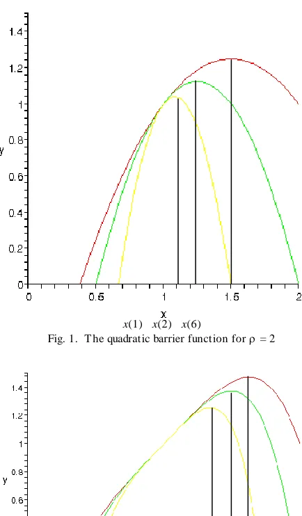
. The barrier terms are formed from a sum of polynomial order of constrained violations and the barrier parameter  determines the amount of the barrier.

The motivation behind the introduction of the polynomial order- term is that they may lead to a representation of an optimal solution of problem (1) in terms of a local unconstrained maximum. Simply stating the definition (2) does not give an adequate impression of the dramatic effects of the imposed barrier. In order to understand the function stated by (2) we give an example with some values for . Some graphs of

B

(

x

,



)

are given in Fig. 13 for the trivial problem

maximize

f

(

x

)



x

subject to

x



1 

0

,

for which the polynomial barrier function is given by

)

,

(

x



B

=

x





(

x



1 )

.

Fig. 1, 2 and 3 depict the one-dimensional variation of the barrier function of  = 2, 4 and 6, for three values of barrier parameter , that is  = 1,  = 2 and  = 6, respectively.

The y-ordinates of these Fig. represent

B

(

x

,



)

for  = 2,  = 4,  = 6, respectively. Clearly, if the solution x * = 1 of this example is compared with the points which maximize

B

(

x

,



)

, it is clear that x * is a limit point of the unconstrained maximizers of

B

(

x

,



)

as .

(2)

112901-7575 IJET-IJENS © February 2011 IJENS

I J E N S

x(1) x(2) x(6)

Fig. 1. T he quadratic barrier function for  = 2

x(1) x(2) x(6)

Fig. 2. T he polynomial barrier function for  = 4

x(1) x(2) x(6)

Fig. 3. T he polynomial barrier function for  = 6

The polynomial barrier method for problem (1) consists of solving a sequence of problems of the form

maximize

B

(

x

,



k

)

subject to

x



0

, (3) where

 



k is a barrier parameter sequence satisfying

1

1 



k





k for all k,



k





.

The method depends for its success on sequentially increasing the barrier parameter to infinity. In this paper, we concentrate on the effect of the barrier parameter.

The rationale for the barrier method is based on the fact

that when



k





, then the term











m

i

i i

k

_A

_x

_b

1

)

(

,

when added to the objective function, tends to infinity if

0 



_i

i

x

b

A

and equals zero if

A

_i

x



b

_i



0

for all

i. Thus, we define the function

f

:

R

n



(



,





]

by



















.

all

for

0 if

,

all

for

0 if

)

(

i

b

x

A

i

b

x

A

x

c

x

f

i i

i i T

The optimal value of the original problem (1) can be written as

f * =

c

T

x

x b Ax , 0

sup

 

=

sup

(

)

0

x

f

x

=

sup

0

lim

(

,

)

k k

x

P



  

. (4)

On the other hand, the barrier method determines, via the sequence of minimizations (3),

)

,

(

sup

lim

k

P

x

f



 



. (5)

Thus, in order for the barrier method to be successful, the original problem should be such that the interchange of “lim” and “sup” in (4) and (5) is valid. Before we give a guarantee for the validity of the interchange, we investigate some properties of the function defined in (2).

First, we derive the concavity behavior of the polynomial barrier function defined by (2) is stated in the following stated theorem.

Theorem 1 (Concavity)

The polynomial barrier function

B

(

x

,



)

is concave in its domain for every  1.

Proof.

It is straightforward to prove concavity of

B

(

x

,



)

using

the concavity of

c

T

x

and -

(

A

_i

x



b

_i

)

. Then the theorem is proven. 

(3)

I J E N S

Theorem 2 (Local and global behavior)

Consider the function

B

(

x

,



)

which is defined in (2). Then

(a)

B

(

x

,



)

has a finite unconstrained maximizer in its domain for every  1 and the set Mof unconstrained maximizers of

B

(

x

,



)

in its domain is compact for every 1.

(b) Any unconstrained local maximizer of

B

(

x

,



)

in its domain is also a global unconstrained maximizer of

)

,

(

x



B

.

Proof.

It follows from Theorem 1 that the smooth function

)

,

(

x



B

achieves its maximum in its domain. We then

conclude that

B

(

x

,



)

has at least one finite unconstrained maximizer.

By Theorem 1

B

(

x

,



)

is concave, so any local maximizer is also a global maximizer. Thus, the set Mof unconstrained maximizers of

B

(

x

,



)

is bounded and closed, because the maximum value of

B

(

x

,



)

is unique, and it follows that M is compact. Theorem 2 has been verified. 

As a consequence of Theorem 2 we derive the monotonicity behaviors of the objective function problem (2), the barrier terms in

B

(

x

,



)

and the maximum value of the polynomial barrier function

B

(

x

,



)

. To do this, for

any



k  1 we denote

x

k and

B

(

x

k

,



k

)

as a maximizer and maximu m value of problem (3), respectively.

Theorem 3 (Monotonicity)

Let

{



k

}

be an increasing sequence of positive barrier parameters such that



k  1 and



k





as

k





. Then

(a)



c

T

x

k



is non-increasing.

(b)













_

_

  m i i k i

x

b

A

1

)

(

is non-increasing.

(c)



B

(

x

k

,



k

)



is non-increasing.

Proof.

Let

x

k and

x

k1 denote the global maximizers of problem (3) for the barrier parameters



k and



k1, respectively. By definition of

x

k and

x

k1 as maximizers and



k 



k1, we have

k k T

x

c







 



m i i k i

x

b

A

1

)

(

≥

_c

T

_x

k1

- k



_

  

_

m i i k

i

x

b

A

1

₎

(

, (6a)

1



k T

_x

c

-



k



  

_

m i i k

i

x

b

A

1 1

₎

(

≥ 1  k T

_x

c

_-

k +1



  

_

m i i k

i

x

b

A

1

₎

(

, (6b)

1



k T

_x

c

- k +1



  

_

m i i k

i

x

b

A

1

₎

(

≥

c

T

x

k -

k +1



 



m i i k i

x

b

A

1

)

(

. (6c)

We multiply the first inequality (6a) with the ratio



k1/

k



, and add the inequality to the inequality (6c) we obtain

1 1 1

1

  































T k

k k k T k k

x

c

x

c



.

Since 0 



k 



k1, it follows that

c

T

x

k



c

T

x

k1 and part (a) is established.

To prove part (b) of the theorem, we add the inequality (6a) to the inequality (6c) to get





_





_

  



 _ _ _ _ m _

i i k i k k m i i k i k k b x A b x A 1 1 1 1 1 ) ( ) (       , thus



  







m i i k i m i i k

i

x

b

A

x

b

A

1 1 1

)

(

)

(

 

as required for part (b).

Using inequalities (6a) and (6b), we obtain

k k T

x

c







 



m i i k i

x

b

A

1

)

(

≥

_c

T

_x

k1

-

k +1



  

_

m i i k

i

x

b

A

1

₎

(

.

Hence, part (c) of the theorem is established. 

We now give the main theorem concerning polynomial barrier method for linear programming problem (1).

Theorem 4 (Convergence of polynomial barrier function) Let

{



k

}

be an increasing sequence of positive barrier parameters such that



k  1 and



k





as

k





. Denote

x

k and

B

(

x

k

,



k

)

as in Theorem 3. Then

(a)

Ax

k



b

as

k





. (b)

c

T

x

k



f

*

as

k





. (c)

B

(

x

k

,



k

)



f

*

as

k





.

Proof.

By definition of

x

k and

B

(

x

k

,



k

)

, we have

k T

_x

(4)

I J E N S Let f * denotes the optimal value of the problem (1). We

have

f * =

c

T

x

x b Ax , 0

sup

 

=

sup

(

,

)

0 k x b Ax

x

B



 .

Hence, by taking the supremum of the right-hand side of (7) over

x



0

and

Ax



b

, we obtain

)

,

(

x

k k

B



=

c

T

x

k -



k



 



m i i k i

x

b

A

1

)

(

≥ f *.

Let

x

be a limit point of

{

x

k

}

. By taking the limit inferior in the above relation and by using the continuity of

x

c

T

and

A

_i

x



b

_i, we obtain

x

c

T -



  



m i i k i k

k

A

x

b

1

)

(

inf

lim



 ≥ f *. (8)

Since



 



m i i k i

x

b

A

1

)

(

 0 and



k





, it follows

that we must have



 



m i i k i

x

b

A

1

)

(



0

and

0 



_i

i

x

b

A

for all i = 1, …, m, 9) otherwise the limit inferior in the left-hand side of (8) will

equal to +. This proves part (a) of the theorem.

Since

{

x



R

n

x



0 }

is a closed set we also obtain that

x



0

. Hence,

x

is feasible, and

f * ≥

c

T

x

. (10) Using (8)-(10), we obtain

f * -



  



m i i k i k

k

A

x

b

1

)

(

inf

lim



 ≥

c

T

x

-



  



m i i k i k

k

A

x

b

1

)

(

inf

lim



 ≥ f *.

Hence,



  



m i i k i k k

b

x

A

f

1

)

(

sin

lim



 = 0

and

f * =

c

T

x

,

which proves that

x

is a global maximum for problem (1). This proves part (b) of the theorem.

To prove part (c), we apply the results of parts (a) and (b),

and then taking

k





of the definition

B

(

x

k

,



k

)

. 

Some notes about this theorem will be taken. First, it assumes that the problem (3) has a global maximum. This may not be true if the objective function of the problem (1) is replaced by a nonlinear function. However, this situation may be handled by choosing appropriate value of . We also note that the constraint

x



0

of the problem (3) is important to ensure that the limit point of the sequence

}

{

_x

k

satisfies the condition

x



0

.

IV. ALGORITHM

The implications of these theorems are remarkably strong. The polynomial barrier function has a finite unconstrained maximizer for every value of the barrier parameter, and every limit point of a maximizing sequence for the barrier function is a constrained maximizer of a problem (1). Thus the algorithm of solving a sequence of maximization problems is suggested. Based on Theorems 4, we formulate an algorithm for solving problem (1).

Algorithm 1

Given Ax = b,



1  0, the number of iteration N and   0. 1. Choose

x

1 

R

nsuch that A

x

1 = b and

x

1  0. 2. If the optimality conditions are satisfied for problem (1)

at

x

1, then stop.

3. Compute

B

(

x

1

,



1

)



max

(

,

1

)

0

B

x



x and the

maximizer

x

1.

4. Compute

B

(

x

k

,



k

)



max

(

,

)

0

k

x

B

x



, the

maximizer

x

k and



k 10



k1 for k = 2.

5. If 

x

k



x

k1  or 

B

(

x

k

,



k

)

–

B

(

x

k1

,



k1

)

  or 

Ax

k



b

 or k = N; then stop.

Else kk + 1 and go to step 4. 

V. INTERIORPOINT ALGORITHM

This section reviews the interiorpoint algorithm called Karmarkar’s algorithm for finding a solution of linear programming problem. The step of this algorithm can be summarized as follows for any iteration (Parwadi, 2011).

Step 1. Given the current initial trial solution

(

x

₁

,

x

₂

,...,

x

_n

)

, set















n

x

D

0

0 .

.

0 ...

0

0 ...

0

0 ...

0

3 2 1 .

Step 2. Calculate

A

~



AD

and

c

~



Dc

.

P



I



A

~

T

(

A

~

A

~

T

)

1

A

~

and

c

_p



P

c

~

.

(5)

I J E N S





p

T

c

x









1

1 ...

1 ~

_,

where  is a selected constant between 0 and 1.

x



D

x

~

as the trial solution for the next iteration (step 1). (If this trial solution is virtually unchanged from the preceding one, then the algorithm has virtually converged to an optimal solution, so stop.)

VI. NUM ERICAL EXAM PLES

This section we give five examples to test the Algoirthm 1 and we compare the results with Karmarkar’s algorithm. Consider the following problems (Parwadi, 2010).

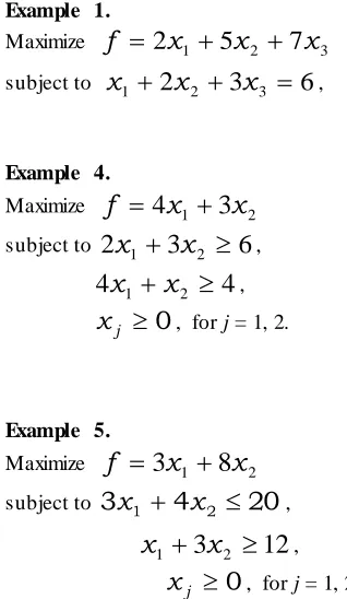
Example 1.

Maximize

f



2 x

₁



5 x

₂



7 x

₃

subject to

x

1



2 x

2



3 x

3



6

,

Example 4.

Maximize

f



4 x

₁



3 x

₂

subject to

2 x

₁



3 x

₂



6

,

4 x

₁



x

₂



4

,

x

_j



0

, for j = 1, 2.

x

j



0

, for j = 1, 2, 3.

Example 2.

Maximize

f



0 .

4 x

₁



0 .

5 x

₂ subject to

0 .

3 x

₁



0 .

1 x

₂



2 .

7

,

0 .

5 x

₁



0 .

5 x

₂



6

,

x

_j



0

, for j = 1, 2.

Example 3.

Maximize

f





3 x

₁



4 x

₂

subject to

x

₁



x

₂



0

,



x

₁



2 x

₂



2

,

x

_j



0

, for j = 1, 2.

Example 5.

Maximize

f



3 x

₁



8 x

₂

subject to

3 x

₁



4 x

₂



20

,

x

₁



3 x

₂



12

,

0 

j

x

, for j = 1, 2.

Table I reports the results of computational for Algorithm 1 ( = 2), Algorithm 1 ( = 4) and Karmarkar’s Algorithm. The first column of Table I contains the example number and the next two columns of each algorithm in this table contain the total iterations and the times (in seconds) of each algorithm.

TABEL I

ALGORITHM 1(=2),ALGORITHM 1(=4) AND KARMARKAR’S ALGORITHM TEST STATISTICS

Problem No.

Algorithm 1( = 2) Algorithm 1( = 4) Karmarkar’s Algorithm

Total Iterations

Time (Secs.)

Total Iterations

Time (Secs.)

Total Iterations

Time (Secs.) 1.

2. 3. 4. 5.

11 8 10 12 15

3.6 4.1 8.8 8.9 10.1

24 8 9 12 20

199.2 77.9 854.6 2960.7 5351.7

16 19 19 12 18

3.6 3.7 3.7 2.8 3.8

Table I also shows that in terms of completion time for the fifth numerical examples, the Algorithm 1 ( = 2) is better than Algorithm 1 ( = 4), but both are still less than the Karmarkar’s algorithm. In terms of the number of iterations required to complete the five numerical examples shows that Algorithm 1 ( = 2) looks better than Karmarkar’s algorithm and Algorithm 1( = 4).

VII. CONCLUSION

As mentioned above, the paper has described the barrier functions with barrier terms in polynomial order- for solving problem (1). The algorithms for these methods are also given in this paper. The Algorithm 1 is used to solve the problem (1). We also note the important thing of these methods which do not need an interior point assumption.

REFERENCES

[1] Durazzi, C. (2000). On the Newton interior-point method for nonlinear programming problems. Journal of Optim ization Theory and Applications. 104(1). pp. 7390.

[2] Kas, P., Klafszky, E., & Malyusz, L. (1999).Convex program based on the Young inequality and its relation to linear programming. Central European Journal for Operations Research. 7(3). pp. 291304.

[3] Parwadi, M., Mohd, I.B., & Ibrahim, N.A. (2002). Solving Bounded LP Problems using Modified Logarithmic-exponential Functions. In Purwanto (Ed.), Proceedings of the National Conference on Mathematics and Its Applications in UM Malang (pp. 135-141). Malang: Department of Mathematics UM Malang.

(6)

International Journal of Engineering & Technology IJET-IJENS Vol: 11 No: 01 50

I J E N S

[5] Parwadi, M. (2011). Some algorithms for solving primal-dual linear programming using barrier methods. International Journal of Mathem atical Archive. 2(1), pp. 108-114. [6] Parwadi, M. (2011). Exponential methods for convex

programming under linear equation constraints. International Journal of Mathem atical Archive. 2(2), pp. 118-129. [7] Wright, S.J. (2001). On the convergence of the Newton/log

-barrier m ethod. Mathematical Programming, 90(1), 71100. [8] Zboo, R.A, Yadav, S.P., & Mohan, C. (1999).Penalty method

for an optimal control problem with equality and inequality constraints. Indian Journal of Pure and Applied Mathem atics. 30(1), pp. 114.