Partial AUC Estimation and Regression

UW Biostatistics Working Paper Series

1-13-2003

Partial AUC Estimation and Regression

Lori E. Dodd

National Institute of Health, [email protected]

Margaret S. Pepe

University of Washington, [email protected]

Suggested Citation

Dodd, Lori E. and Pepe, Margaret S., "Partial AUC Estimation and Regression" ( January 2003).UW Biostatistics Working Paper Series.

1. Introduction

Screening and diagnostic tests are familiar and ever-evolving tools of modern medicine. Popu-lations of healthy individuals characterized as at-risk are commonly screened for diseases such as cancer and heart disease. Early detection by screening is considered essential to alleviate dis-ease burden, and considerable resources have been devoted to developing new screening tests. New diagnostic tests that are less invasive, less expensive, and more accurate than existing procedures are sought for diagnosis of many conditions. Technologies that measure gene and protein expression, as well as new imaging procedures all hold promise in this regard. Prior to wide-spread application, however, rigorous evaluation of test accuracy and of factors that effect it is compulsory.

Inherent in the analysis of screening and diagnostic tests are costs and benefits, both mon-etary and non-monmon-etary, associated with true positive and false positive diagnoses. Consider a continuous test result Y for which Y > c indicates a positive test result, and D and D de-note diseased and non-diseased states, respectively. The true positive rate at a threshold c,

T P R(c), is defined as P(Y > c | D)≡S_D(c). The corresponding false positive rate, F P R(c), isP(Y > c|D)≡S_D(c). Costs and benefits are associated with any given{F P R(c), T P R(c)} pair. The Receiver-Operating Characteristic (ROC) curve plots{F P R(c), T P R(c)}for all pos-sible thresholds c, and provides a visual description of the trade-offs between TPRs and FPRs as one changes the threshold stringency (Figure 1). We can write the ROC curve as a function of t = S_D(c) as follows: ROC(t) = S_D{S−1

D (t)}. An uninformative test is represented by a

straight line from the (0,0) vertex to (1,1), while a curve pulled closer towards the (0,1) vertex indicates a better performing test.

Frequently, the best threshold is not known when a test is under evaluation, and it may vary depending on the setting in which the test is implemented. A summary measure that aggregates performance information across a range of possible thresholds is desirable. The area

under the ROC curve (AUC), defined as₀1ROC(t)dt,summarizes across all thresholds, and is the most commonly used measure of diagnostic accuracy for quantitative tests. However, the AUC summarizes test performance over regions of the ROC space in which one would never operate, i.e., for {F P R(c), T P R(c)} values of no practical interest. In population screening, large monetary costs result from high false positive rates; hence the region of the curve corre-sponding to low false positive rates is of primary interest. In diagnostic testing, it is critical to maintain a high TPR in order not to miss detecting subjects with disease. In this case, interest is in the region of the ROC curve corresponding only to acceptable high TPRs. In this paper, we consider a summary index for the ROC curve restricted to a clinically relevant range of false positive rates. The partial AUC is

AU C(t₀, t₁) =

_t1 t0

ROC(t)dt, (1)

where the interval (t₀, t₁) denotes the false positive rates of interest. The analogue that restricts to a range of true positive rates will also be discussed. Selecting the interval (t₀, t₁) is an important practical issue. The choice depends on the particular setting and should depend on the costs of a false positive diagnosis as well as the benefits of a true positive. Baker (2000) develops a “utility” function to specify a target partial ROC region. Obuchowski (1997) uses decision analysis to associate patient outcome with desirable diagnostic accuracy values. Such methods could be adapted, for example, to determine a maximum allowable false positive rate or the lowest desirable true positive rate. This is a complex area requiring input from health services and economic specialists.

Although the partial AUC has been proposed before (McClish, 1989; Thompson and Zuc-chini, 1989; Jiang et al., 1989) and has gained popularity, particularly in screening research (Baker and Pinsky, 2001), little attention has been devoted to statistical inference about it. We provide a probabilistic interpretation for the partial AUC that gives rise to a novel non-parametric estimator. Through simulation studies, the estimator is compared with the existing

estimators that are all based on parametric assumptions. We show that the increased robust-ness of the non-parametric estimator is gained at the expense of a moderate loss in efficiency. Next, we present a regression framework for evaluating covariate effects on the partial AUC. The approach extends a method developed recently for regression analysis of the full AUC (Dodd and Pepe, 2003). Since the partial AUC has more appeal in many practical settings, this represents an important generalization.

The work is motivated by a study of prostate-specific antigen (PSA), a serum biomarker. PSA is a screening tool for prostate cancer that has been the focus of much research. Important questions to consider when evaluating this biomarker are: Which form of PSA is best (total or ratio of free to total PSA)? and, by how long does this test advance the lead time, or time prior to clinical diagnosis of disease? In this paper, we show that a parsimonious regression model of the partial AUC with PSA type and lead time as covariates assists with this type of evaluation.

2. Partial AUC

The partial AUC is simply the area under the ROC curve betweent₀ andt₁ (Figure 1). With an uninformative test, T P R(c) =F P R(c) for allc, and the partial AUC is the area of a trapezoid equal to 1₂(t₁ +t₀)(t₁−t₀). For a perfect test, ROC(t) = 1 for all t ∈ (0,1), and the partial AUC is the area of the rectangle with height 1 and baset₁−t₀.

INSERT FIGURE 1 ABOUT HERE. 2.1 Interpretations of the Partial AUC

Assume YD and YD are continuous random variables with survivor functions S_D and S_D, respectively. LetF = 1−S. The partial AUC is the joint probability that YD > YD and that

AU C(t₀, t₁) = _t1 t0 ROC(t)dt = _t1 t0 S_D(S−1 D (t))dt = _S−1 D (t0) S_D−1(t1) S_D(y)dF_D(y) = _S−1 D (t0) S−1 D (t1) S_D(y)f_D(y)dy = P YD > YD, YD ∈ {S−1 D (t1), SD−1(t0)} (2) To simplify notation let q₀ = S−1

D (t0) and q1 = SD−1(t1). The partial AUC can also be written

as a weighted conditional expectationAU C(t₀, t₁) = (t₁ −t₀)P

YD > YD|YD ∈(q₁, q₀)

.

A second interpretation arises from the concept of placement values (Pepe, 2003). Hanley and Hajian-Tilaki (1997) showed a connection between average placement values and the full AUC. We extend their result to the partial AUC here, as it provides an interesting interpretation of the partial AUC as well as a simpler estimator:

P YD > YD, YD ∈(q₁, q₀)|YD =yD = P YD > yD, yD ∈(q₁, q₀) = I yD ∈(q₁, q₀) P YD > yD = I yD ∈(q₁, q₀) S_D(yD) ≡ P lD(yD) (3)

We refer to P lD(yD) as a restricted placement value (with respect to the distribution of results from the diseased population). Note that a full placement value is defined as in (3) except there is no restriction toYD ∈(q₀, q₁). The termS_D(yD) is theplacement of a given non-diseased test result,YD =yD, in the survivor function of results of diseased. For a good test, the non-diseased observations fall in the lower tail of the distribution of diseased. Hence, larger placement values indicate a better test. The restricted placement is weighted so that only those values that fall

within the relevant quantiles are considered. Note thatE{P lD(YD)}=AU C(t₀, t₁). Thus, the partial AUC can be thought of as an average of restricted placement values. It is straightforward to show that the partial AUC is also the expected restricted placement value which conditions on observations from the diseased population.

One may wish to rescale the partial AUC, especially in regression analysis (see Section 6). We define the partial AUC odds as:

AU C(t₀, t₁) (t₁−t₀)−AU C(t₀, t₁) = P{YD > YD|YD ∈(q₁, q₀)}(t₁−t₀) 1−P{YD > YD|YD ∈(q₁, q₀)}(t₁ −t₀) = P{Y D _{> Y}D_|YD _∈(q 1, q0)} P{YD < YD|YD ∈(q₁, q₀)}. (4) This is the ratio of the probability of a correct ordering of a randomly selected diseased and non-diseased test result to the probability of an incorrect ordering, with both probabilities

conditional on the test result of non-diseased arising from the region of interest. These odds have value of t1+t0

2−(t1+t0)when a test is uninformative and of infinity for a perfect test. 2.2 Restricting the True Positive Range

The partial AUC just described restricts the ROC region of interest to false positive rates that take values in (t₀, t₁). In some settings, one may wish to restrict to a range of true positive rates (Jiang et al., 1996). By transforming the ROC curve to a plot of {S_D(c),1−S_D(c)}, interpretations of a partial AUC corresponding to true positive rates in an interval are easily obtained. The curve is no longer the classic ROC curve. It is simply a 270◦rotation of Figure 1. We refer to this curve as the Specificity-ROC curve (ROC_spe) since specificity is plotted on the y-axis. Foru=S_D(c), this curve is described byROC_spe(u) = 1−S_D{S_D−1(u)}=F_D{S_D−1(u)}. The partial AUC for a range of true positives, denotedAU CT P(u₀, u₁), is defined as:

_u1 u0 ROC_spe(u)du = _S−1 D (u1) S−1 D (u0) {1−S_D(y)}dS_D(y) = P YD > YD, YD ∈ {S_D−1(u₁), S_D−1(u₀)} . (5)

Note that₀1S_D(y)dS_D(y) =₀1{1−S_D(y)}S_D(y). Therefore, the two representations give the same fullAU C. However, the quantiles that define the partial AUC are{S−1

D (t1), SD−1(t0)},

and are derived from the non-diseased distribution for the classic ROC curve. For the case just presented the quantiles are {S_D−1(u₁), S_D−1(u₀)}, and arise from the distribution of tests of diseased subjects. With this exception, the interpretations are the same. Thus, we focus on the classic ROC curve, recognizing that methods developed here easily extend to the case in which restriction of true positive rates is required.

3. Estimators

3.1 Parametric Estimators

Before proposing our non-parametric estimator, we briefly describe existing estimators. Mc-Clish (1989) describes what we refer to as the normal distributions partial AUC estimator (NDE), which assumes that the test results for diseased and non-diseased populations follow normal distributions with different means and variances. Maximum likelihood estimates of these parameters provide the ROC curve estimate, and numerical integration of it gives the partial AUC estimator: AU C (t₀, t₁) = _tt1

0 Φ a+bΦ−1(t) dt. Here a = (µ_D −µ_D)/σ_D and

_{b=σD/σD, where µ and σ}2 _{denote mean and variance, respectively.}

Another approach is to parameterize the ROC curve directly. The most common form is the binormal ROC curve, ROC(t) = Φ{a+bΦ−1(t)}, for which the partial AUC is given by the same formula above. However, because this approach does not parameterize the distributions of test results, but only the ROC curve that describes the relationship between their distribu-tions, it stipulates far weaker assumptions. Two methods have been proposed for estimating parameters a and b of the binormal ROC curve (Pepe, 2000; Metz, Herman, and Shen, 1998). Both methods are distribution free in that they are functions only of the ranks of the data.

3.2 Proposed Non-Parametric Estimator

Denote V_ijq0,q1 = I{Y_iD > Y_jD, Y_jD ∈ (q₁, q₀)}, and observe that EV_ijq0,q1 = P{YD > YD, YD ∈ (q₁, q₀)} = AU C(t₀, t₁), according to the interpretation of equation (1). This suggests the following method of moments estimator:

AU C(t₀, t₁) = 1 n_Dn_D ij V_ijq0,q1. (6)

In some circumstances the quantiles (q₀, q₁) will be known. In others, they will not, in which case, empirical quantile estimates are substituted. If the empirical quantile value does not coincide precisely with the desired value, as may happen with small sample sizes, values are linearly interpolated. Observe that, when t₀ = 0 and t₁ = 1, AU C (t₀, t₁) = _n 1

DnD

ijI(YiD >

Y_jD). Hence, for the full AUC the estimator reduces to the Mann-Whitney U-statistic, the classic non-parametric AUC estimator. Further, note that this results in the same value as the area calculated from the empirical ROC curve using the trapezoidal rule when there are no ties in the data.

The same estimator is derived by consideration of empirical restricted placement values. Let

S denote an empirical survivor function and write the empirical placement value corresponding to an observation from a disease-free subject, YD, as:

P lD(Y_jD) = I Y_jD ∈(q₁, q₀) S_D(Y_jD) = I Y_jD ∈(q₁, q₀) ₁ n_D nD i I(Y_iD > Y_jD). (7) The sample average is

1 n_D n_D j P lD(Y_jD) = 1 n_Dn_D n_D j nD i I Y_iD > Y_jD, Y_jD ∈(q₁, q₀) .

Thus, the non-parametric estimator is an average of partial AUC placement values within the disease reference distribution. Likewise, the estimator can be written as the average of the

placement values within the non-diseased reference distribution. This generalizes the corre-sponding results for the full AUC given in DeLong, DeLong and Clarke-Pearson (1988) and Hanley and Hajian-Tilaki (1997). Calculations using placement values are considerably faster computationally, and are used in the simulations described next.

Asymptotic distribution theory is non-standard because the binary indicators, V_ijq0,q1, are cross-correlated. It can be shown that the projection _n 1

DnD

ijP lD(YiD)+P lD(YjD) is

asymp-totically equivalent to (6). Since this projection is a sum of independent terms, standard theory provides consistency and asymptotic normality results. For complete details, refer to Dodd (2001). We recommend using the bootstrap to obtain variance estimates.

4. Simulations

4.1 Small Sample Performance of the Estimator

Three different ROC models were simulated to evaluate performance of the proposed method of inference. The models simulated are a normal distributions model, a proportional hazards ROC model, and an extreme value ROC model. The proportional hazards ROC model assumes that the hazard function for the disease test result distribution is proportional to that of the non-disease distribution. If the ratio of hazards is r, then ROC(t) = tr. The extreme value ROC model involves two parameters (e, f), and is of the formROC(t) = exp[−1_e exp{−fΦ−1(t)}] (Cai and Pepe, 2003). Briefly, extensive simulations of these models described in Dodd(2001) showed that the non-parametric method produced estimates with little bias and that confidence intervals using the bootstrap standard error estimator and normal quantiles provided good coverage probability.

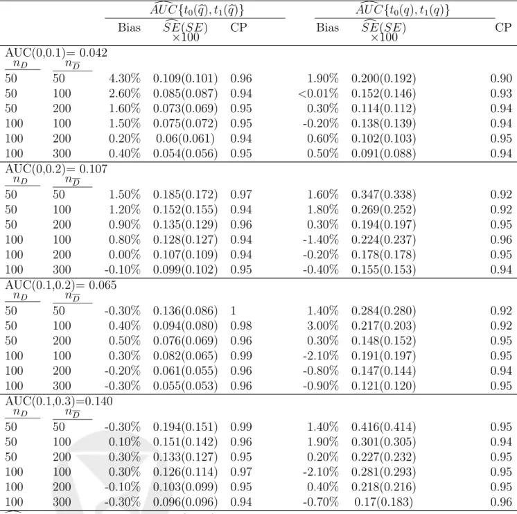
We present results for the normal distributions model here. This assumesYD ∼N(1.5,1.44) and YD ∼N(0,1) (see Figure 1). Partial AUCs are considered for (t₀, t₁) = {(0,0.1), (0,0.2), (0.1,0.2), (0.1,0.3)} when quantiles are both known and estimated empirically. Sample sizes were generated with both equal and unequal numbers in each group, such that (n_D, n_D)=

{(50,50),(50,100), (50,200), (100,100),(100,200), (100,300)}. All resulted in estimates with little bias. The largest amount of bias (4.3%) occurs for a sample size of 50 per group for (t₀, t₁) = (0,0.1) when empirical quantiles are used. Bias becomes negligible as sample size increases and as more of the curve is integrated.

Bootstrapped standard errors, computed with 200 bootstrap samples, overestimate the truth somewhat when the quantiles are estimated. In the case when quantiles are known, the boot-strapped standard error estimator is reasonably unbiased. Consequently, confidence interval coverage tends to be above the nominal level with estimated quantile values, but close to the nominal level with the known threshold. Surprisingly, when empirical quantiles are substi-tuted, there is an increase in efficiency relative to the case when the true quantile is used. The true standard errors associated with AU C {t₀(q), t₁(q)} are consistently smaller than those for

AU C{t₀(q), t₁(q)}. The reason for this is unclear to us, but it is a real phenomenon observed throughout our simulation studies.

4.2 Robustness

To investigate if the non-parametric estimator gains robustness over other estimators, we considered settings where the ROC curve deviated from the classic binormal form. We gen-erate an ROC model in which test results arise from mixtures of distributions. Assume that YD ∼ N(0,1), but that YD is a mixture of two normal distributions, f_Z1 and f_Z2, with Z₁ ∼ N(µ_D,1, σ_D,2 ₁) and Z₂ ∼ N(µ_D,2, σ_D,2 ₂), such that the probability density of YD

is p f_Z1(y) + (1−p) f_Z2(y), for a mixing proportion p∈(0,1). The resulting ROC curves are simply mixtures of ROC curves weighted by the appropriate mixing probabilities and can be expressed asROC(t) =pΦ(a₁+b₁Φ−1(t)) + (1−p)Φ(a₂+b₂Φ−1(t)), where a_i = µD,i_σ−µD,i

D,i and

b_i = σ_σD,i

D,i for i = 1,2. We set µD1 = 5, σ

2

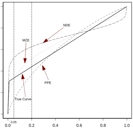
D1 = 1.2, µD2 = 0, σ2D2 = 1, and p = 0.3. The true ROC curve is the solid line shown in Figure 2. We use t₀ = 0 and three separate maximum false positive rates, t₁ = 0.05,0.1,1.0. Very low false positive rates such as t₁ = 0.05 have been

advocated in settings such as cancer screening (Baker and Pinsky, 2001). INSERT FIGURE 2 ABOUT HERE

Estimates of ROC curves from the normal distributions estimator (NDE), the Pepe estimator (PPE) and the Metz estimator (MZE) are also given in Figure 2. Recall that the normal distributions estimator assumes that test results are normally distributed in diseased and non-diseased populations, and, using sample means and variances, the ROC curve is calculated as

ROC(t) = Φ{a+bΦ−1(t)} with a = µ0D−µ0D 0 σD and b = 0 σ_D 0

σD. Clearly, all of these curves fail to

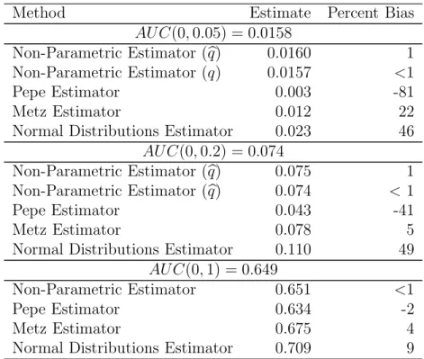
accurately represent the true curve which is not of the binormal form. They parameterize the ROC curve incorrectly, and hence, produce biased partial AUC estimates (Table 2). The largest bias was observed with the normal distributions estimator. In contrast to this estimator and those of Pepe and Metz, the non-parametric estimators produce estimates with very small bias. Observe that the amount of bias decreases for both the Metz and the Pepe estimators as more of the curve is integrated. This is consistent with results showing that the binormal model estimators produce AUC estimates which are robust to departures from this model (Hanley, 1996).

Additionally, note that the non-parametric methods model and estimate the ROC over the entire (0,1) range and then integrate the relevant portion to determine the partial AUC. On the other hand, the proposed methoddirectly estimates the partial AUC over the false positive rate range of interest. A more robust approach might be to model over (t₀, t₁), which can be accomodated by the Pepe approach. When the estimates are computed restricting to (0,0.05) and (0,0.2), however, there is still bias with the Pepe method. The mean estimates restricting to the corresponding intervals are AU C (0,0.05) = 0.013 (-18% bias) and AU C (0,0.2) = 0.044 (-40% bias).

4.3 Efficiency

We compare the efficiency of the methods for estimating the partial AUC under the normal distributions model. In this setting, the normal distributions estimator is more efficient than the others as it is the maximum likelihood estimator and makes use of the information that the data are normally distributed. The results presented in Figure 3 indicate that the non-parametric estimator with known quantile, N P E(q), is the least efficient of the methods. In agreement with Table 1, we observe that the non-parametric estimator is more efficient when the quantile is estimated than when the known value is used. The distribution-free binormal estimators are more efficient than the non-parametric estimator but have reduced efficiency relative to the approach that models the test results. Although very similar, the Pepe estimator appears to be slightly more efficient than the Metz estimator.

The efficiency of all methods approaches that of the normal distributions estimator ast→1. Recall that when t = 1, the non-parametric estimator is the Mann-Whitney U-statistic. The normal distributions estimator is simply a transformation of the standardized differences in means, i.e., of the Z-statistic. Hence, the comparison of the variance of the non-parametric estimator with the variance of the normal distributions estimator is akin to the comparison of the efficiency of the Mann-Whitney U-statistic to that of the Z-statistic. It is well known that the asymptotic relative efficiency of the Mann-Whitney U-statistic to the t-statistic is 0.95 Lehmann (1997). Thus, it is no surprise that, in this study, the relative efficiency is 0.94 att = 1.

INSERT FIGURE 3 ABOUT HERE 4.4 Recommendations

The normal distributions estimator, while most efficient, produces unacceptably biased es-timates. Estimators that parameterize the ROC curve are similarly not robust. The non-parametric estimator provides substantially more robust estimation. The added robustness is

at the expense of moderate losses in efficiency. Hence, we recommend use of the non-parametric estimator. Indeed, for partial areas witht >0.1, it has similar efficiency to the Pepe and Metz methods.

5. Regression Analysis

Accuracy may depend on information other than the test result itself. For example, accuracy may depend on how close in time a subject is to clinical diagnosis. Patient characteristics such as age or family history of disease may also be relevant determinants of accuracy. This information may guide decisions about which populations are most likely to benefit from testing or for which populations test innovations are needed. We extend regression methodology we previously developed for the AUC to a regression methodology for the partial AUC summary index of test accuracy. For a more extensive discussion of modelling approaches for the AUC and details about fitting, refer to Dodd and Pepe (2003). Here, we elaborate only on aspects unique to the partial AUC.

5.1 Models

To assess the effect of covariates on test accuracy, we propose the following partial AUC regression models. Consider a vector of covariatesX. Define the covariate-specific partial AUC as AU C_X(t₀, t₁) = P(YD > YD, YD ∈ (q₀, q₁)|X). For a specified link function g, the general model is given by:

AU C_X(t₀, t₁) =g(XTβ) (8) Possible link functions include the logit or probit forms. However, since AU C(t₀, t₁) has an upper bound of (t₁ − t₀), a generalization of the logit that incorporates this constraint is appropriate:g−1(u, t₀, t₁) = log_(t u

1−t0)−u. When this link is used an interpretation that cor-responds to the partial AUC odds defined earlier follows. Consider the model:

log AU C_X(t₀, t₁) (t₁−t₀)−AU C_X(t₀, t₁) =β₀+β₁X. (9)

It follows that eβ1 _{is a ratio of partial AUC odds for X+ 1 to X. When e}β1 _{> 1, the partial} AUC odds are an increasing function of X, and accuracy increases with X. If eβ1 _{< 1, the} partial AUC odds are a decreasing function of X. Refer to Dodd and Pepe (2003) for details about model specification.

5.2 Estimating Function

Consider the indicators V_ij(q0,q1) as defined in (6), but now we condition on the covariates

X. They have mean E

V_ij(q0,q1)| X

= AU C_X(t₀, t₁), which suggests that binary regression methods can be used to estimate partial AUC model parameters with the following estimating equation: V_nD,nD(β) = nD i n_D j ∂θ_X ∂β ν −1_(θ X) V_ij(q0,q1)−θ_X = 0. (10)

Here, θ_X =AU C_X(t₀, t₁), ν−1(θ_X) is the variance ofV(q0,q1)_{, and} ∂θX

∂β is a (p×1) vector of the

partial derivatives of θ_X with respect to the model parameters β. This resembles the classic estimating equation for binary regression. However, the binary indicators are cross-correlated, in the sense that, for a given i the set of binary variables {V_ij, j = 1, ..., n_D} are correlated because they are a function of Y_iD. Consistency and asymptotic normality for parameter es-timates from a similar estimating equation is developed in Dodd and Pepe (2003). The same theory applies here, at least when the quantiles (q₀, q₁) are known. See Dodd (2001) for full exposition.

5.3 Comparing two tests

The proposed estimating equation gives rise to a standard approach when a model to compare two tests is of interest. Consider the following model: log[AU C_X(t₀, t₁)/{t₁ −t₀ − AU C_X(t₀, t₁)}] =β₀+β₁X, where X is an indicator of test type. The score-like test of β₁ = 0, based on the estimating equation in (10), reduces to AU C _X=1(t₀, t₁)−AU C _X=0(t₀, t₁), where

by Wieand et al. (1989) that takes integrated differences in weighted ROC curves to compare two tests. The Wieand et al. approach does not require bootstrapping for inference as does ours when the quantiles, q₀ and q₁, are unknown. The current approach, on the other hand, provides a more general regression framework.

5.4 Implementation

To obtain parameter estimates, algorithms developed for binary regression are used. First, however, the quantiles (q₀, q₁) must be specified. If known, they are simply substituted into (10). If quantiles are unknown and do not depend on covariates, they can be estimated empirically from the non-disease data at hand. If the unknown quantiles depend on covariates, a quantile regression model may be specified. Then, the binary indicators based on pairs of diseased and non-diseased observations are computed. When covariates are categorical and there are sufficient observations of diseased and non-diseased within each category, all possible pairs of diseased and non-diseased within a given category are created. That is, the nk_D and nk

D

observations corresponding to the category or level of covariate k are selected and we calculate

V_ij(q0,q1) at eachX fork = 1, ..., K. Note that the estimating function is modified to indicate the sum overk. When covariates are continuous, pairing of diseased and non-diseased observations (Y_iD, Y_jD) may be undertaken for all possible pairs, although we prefer to pair those observations only with covariate values near one another. Finally, if covariates are unique to the diseased group, as with the “time prior to diagnosis” covariate in the PSA example that follows, the covariate does not restrict the pairing. Pairing is based only on covariates common to D and

D. We refer to the paper on AUC regression by Dodd and Pepe (2003) for a detailed discussion of pairing in the presence of covariates. The same considerations are relevant here.

Logistic or probit regression estimation routines in standard statistical packages can be used to solve the estimating equations. Note that standard errors reported from these packages will not be valid, even with a robust sandwich variance estimator because of the crossed-correlation

structure. We use the bootstrap to calculate the standard errors for parameter estimates. Bootstrap samples are taken by sampling subjects as the primary unit.

6. Prostate-Specific Antigen Analysis

The data analyzed here are taken from a retrospective sampling of stored serum from the α -Tocopherol and β-Carotene Study (ATBC), described by Heinonen et al. (1998). Although the primary goal of this study was to evaluate the effect of dietary supplementation of α -Tocopherol and β-Carotene on lung cancer risk, the development of prostate cancer was also recorded. Additionally, serum samples were collected and stored at baseline and three years later. For those 240 subjects who were diagnosed with prostate cancer during the eight-year follow-up period, their serum samples were retrospectively evaluated for pre-diagnostic levels of prostate-specific antigen. Age-matched serum samples for 237 non-prostate diagnosed subjects were selected for comparative purposes. Two ways of quantifying PSA were considered, the total PSA in serum (denoted by Total) and the ratio of free to total PSA in serum (denoted by Ratio). Etzioni et al. (1999) previously compared these two measures using a different dataset. In addition to comparing Total with Ratio PSA, we examine the effect of time from serum sampling to clinical diagnosis on accuracy. One would expect that PSA levels taken close to the time of clinical time of diagnosis would be more predictive. Let test denote an indicator that takes a value of one for total PSA and zero for PSA ratio. The term time denotes years prior to clinical diagnosis at which PSA was measured, so that ‘−7’ indicates ‘7 years before diagnosis’ and ‘0’ indicates sampling concurrent with diagnosis.

Studies of the false positive rates of PSA at the standard threshold of 4.0 ng/mL vary widely, with values ranging from 0.10 to 0.70 reported in the literature (Tanguay et al., 2002; Barry, 2001). We consider the following partial AUC regression model fromt₀ = 0 to the midpoint of

reported false positive rates, i.e., t₁ = 0.4: log AU C(0,0.4)

0.4−AU C(0,0.4) =β0+β1test+β2time+β3test∗time. (11) The “time” covariate is irrelevant in the disease-free group, hence 1−tth₁ empirical quantile within each test type was substituted forq₁. Refer to Table 3 for parameter estimates. Bootstrap sampling was conducted with 200 replicates using case-control sampling with subjects as the primary unit. In accordance with Etzioni’s results, Total PSA appears to be the better marker for prostate cancer. Attime= 0, the partial AUC odds ratio is 2.67 which is almost statistically significant at 5% (p= 0.07). As expected, PSA accuracy improves when subjects are measured at times closer to clinical diagnosis of prostate cancer. Although this is true for both measures, the interaction term indicates that the time effect is different for the two measures. There is a 17% greater increase in partial AUC odds for each year for total PSA relative to ratio PSA. For total PSA, the partial AUC odds increase by about 23% for year closer to diagnosis, while, for ratio the partial AUC odds only increase by 5% for each year. Stated another way, the relative performance of the measures changes with time. The relative odds, estimated as 2.67 at diagnosis, is 1.4 at four years prior to diagnosis (Figure 4). Figure 4 also plots the fitted model. Empirical partial AUCs are averaged within a time window, where intervals are selected so that there were sufficient observations per window, while avoiding wide time intervals. The model appears to give a reasonable fit, as the fitted and empirical lines are fairly close.

INSERT FIGURE 4 ABOUT HERE

7. Discussion

The partial AUC summarizes test accuracy over a clinically relevant region of the ROC curve. This summary measure can be interpreted as a joint probability thatYD > YD and thatYD lies within the quantiles corresponding to the relevant false positive region. Similarly, the measure can be thought of as the expected restricted placement value. These related interpretations

give rise to a new, non-parametric partial AUC estimator that is more robust than existing estimators, and loses only moderate efficiency relative to them. Simulation studies demonstrate reasonable performance of the approach under a range of models. Interestingly, the estimator is more efficient when estimated quantiles are substituted, as opposed to using their true values. When true quantiles are known, one may prefer to estimate them for a gain in efficiency.

We extend the approach to making inference about partial AUC regression models. One could also use the Derived Variables approach, as proposed by Thompson and Zucchini (1989) or modify the Jackknifed-AUC approach of Dorfman et al. (1992) for regression modelling. These methods have been shown to be less efficient in previous studies ( Dodd and Pepe (2003)). Further, they are not sufficiently flexible for the range of models of scientific relevance. For example, neither of these methods could be applied to the PSA analysis presented because the time prior to diagnosis covariate is continuous, and these other methods are restricted to discrete covariate types.

Lastly, we emphasize that, although the partial AUC estimator is a more clinically relevant summary measure of accuracy, the choice of the appropriate restricted region may be arguable. More research is necessary to provide guidance for determining the relevant region. Such a method would inevitably depend on information about the costs and benefits associated with true and false positive diagnoses.

8. Acknowledgements

Research supported by Grants T32 HL07183 and R01 GM54438 from the NIH.

References

Baker, S. (2000). Indentifying combinations of cancer markers for further study as triggers of early intervention. Biometrics 56, 1082–1087.

Baker, S. and Pinsky, P. (2001). A proposed design and analysis for comparing digital and ana-log mammography: Special receiver operating characteristic methods for cancer screening.

Journal of the American Statistical Association 96, 421–428.

Barry, M. (2001). Prostate-specific-antigen testing for early diagnosis of prostate cancer. New England Journal of Medicine 344, 1373–1377.

Cai, T. and Pepe, M. (2003). Semi-parametric_ROCanalysis to evaluate biomarkers for disease.

Journal of the American Statistical Association 97, 1099–1107.

DeLong, E. R., DeLong, D. and Clarke-Pearson, D. (1988). Comparing the areas under two or more correlated receiver operating characteristic curves: a nonparametric approach. Bio-metrics 44, 837–845.

Dodd, L. (2001). Regression Methods for Areas and Partial Areas Under the Receiver-Operating Characteristic Curve. PhD thesis, University of Washington, Seattle, WA 98195.

Dodd, L. and Pepe, M. (2003). Semi-parametric regression for the area under the receiver operating characteristic curve. Journal of the American Statistical Association , in press. Dorfman, D., Berbaum, K. and Metz, C. (1992). Receiver operating characteristic analysis:

generalization to the population of readers and patients with the jackknife method. Inves-tigative Radiology 27, 723–731.

Etzioni, R., Pepe, M., Longton, G., Hu, C. and Goodman, G. (1999). Incorporating the time diminsion in receiver operating characteristic curves. Medical Decision Making 19, 242–251. Hanley, J. and Hajian-Tilaki, K. (1997). Sampling variability of nonparametric estimates of the areas under receiver operating characteristic curves: An update. Academic Radiology

17, 49–58.

Heinonen, O., Albanes, D., Vitarmo, J. and Taylor, P. (1998). Prostate cancer and supple-mentation with α-tocopherol and β-carotene: Incidence and mortality in a controlled trial.

Lehmann, E. (1997). Testing Statistical Hypotheses, chapter 6, pages 314–321. Springer-Verlag. McClish, D. (1989). Analyzing a portion of the _ROC curve. Medical Decision Making 9,

190–195.

Metz, C., Herman, B. and Shen, J.-H. (1998). Maximum likelihood estimation of receiver operating characteristic (_ROC) curves from continuously-distributed data. Statistics in Medicine 17, 1033–1053.

Obuchowski, N. (1997). Testing for equivalence of diagnostic tests. American Journal of Roentgenology 168, 13–17.

Pepe, M. (2000). An interpretation for the _ROC curve and inference using _GLM procedures.

Biometrics 56, 352–359.

Pepe, M. (2003). Statistical Evaluation of Medical Tests for Classification and Prediction. Oxford University Press.

Tanguay, S., Begin, L., Elhilali, H., Karakiewicz, P. and Aprikian, A. (2002). Comparative evaluation of total_PSA, free/total_PSA, and complexed_PSAin prostate cancer detection.

Adult Urology 59, 261–265.

Thompson, M. L. and Zucchini, W. (1989). On the statistical analysis of_ROCcurves. Statistics in Medicine 8, 1277–1290.

Wieand, S., Gail, M., James, B. and James, K. (1989). A family of nonparametric statistics for comparing diagnostic markers with paired or unpaired data. Biometrika76, 585–92.

FPR TPR 0.0 0.2 0.4 0.6 0.8 1.0 0.0 0.2 0.4 0.6 0.8 1.0 t0=0.1 t1=0.3

Rectangle: Perfect Test

Trapezoid: Uninformative Test

0.0 0.2 0.4 0.6 0.8 1.0 FPR 0.0 0.2 0.4 0.6 0.8 1.0 TPR NDE 0.05 True Curve PPE MZE

Figure 2. Estimates of the ROC based on data from the mixture model. Shown are curves

that use the average parameter estimates. NDE: Normal Distributions Estimator. PPE: Pepe Estimator. MZE: Metz Estimator.

Maximum False Positive Rate Relative Efficiency 0.0 0.2 0.4 0.6 0.8 1.0 0.0 0.2 0.4 0.6 0.8 1.0 t=0.01 NPE(q) NPE( q ) PPE MZE >

Figure 3. Efficiency of Estimators Relative to the maximum likelihood Normal Distributions

Estimator. Shown are results with sample sizes of 200 per group and 2,000 replicates per scenario.

Total PSA

Ratio PSA

-7 -6 -5 -4 -3 -2 -1

Years Prior to Clinical Diagnosis

0.26 0.28 0.30 0.32 0.34 AUC(0,0.4)

Figure 4. AU C(0,0.4) Model Fit. Solid lines represent fitted model. Dotted lines represent empirical values averaged over a time window.

Table 1: Bias and Coverage Probability of the Non-Parametric Method with known and estimated quantiles. AU C{t₀(q), t₁(q)} AU C {t₀(q), t₁(q)} Bias SE(SE) CP Bias SE(SE) CP ×100 ×100 AUC(0,0.1)= 0.042 n_D n_D 50 50 4.30% 0.109(0.101) 0.96 1.90% 0.200(0.192) 0.90 50 100 2.60% 0.085(0.087) 0.94 <0.01% 0.152(0.146) 0.93 50 200 1.60% 0.073(0.069) 0.95 0.30% 0.114(0.112) 0.94 100 100 1.50% 0.075(0.072) 0.95 -0.20% 0.138(0.139) 0.94 100 200 0.20% 0.06(0.061) 0.94 0.60% 0.102(0.103) 0.95 100 300 0.40% 0.054(0.056) 0.95 0.50% 0.091(0.088) 0.94 AUC(0,0.2)= 0.107 n_D n_D 50 50 1.50% 0.185(0.172) 0.97 1.60% 0.347(0.338) 0.92 50 100 1.20% 0.152(0.155) 0.94 1.80% 0.269(0.252) 0.92 50 200 0.90% 0.135(0.129) 0.96 0.30% 0.194(0.197) 0.95 100 100 0.80% 0.128(0.127) 0.94 -1.40% 0.224(0.237) 0.96 100 200 0.00% 0.107(0.109) 0.94 -0.20% 0.178(0.178) 0.95 100 300 -0.10% 0.099(0.102) 0.95 -0.40% 0.155(0.153) 0.94 AUC(0.1,0.2)= 0.065 n_D n_D 50 50 -0.30% 0.136(0.086) 1 1.40% 0.284(0.280) 0.92 50 100 0.40% 0.094(0.080) 0.98 3.00% 0.217(0.203) 0.92 50 200 0.50% 0.076(0.069) 0.96 0.30% 0.148(0.152) 0.95 100 100 0.30% 0.082(0.065) 0.99 -2.10% 0.191(0.197) 0.95 100 200 -0.20% 0.061(0.055) 0.96 -0.80% 0.147(0.144) 0.94 100 300 -0.30% 0.055(0.053) 0.96 -0.90% 0.121(0.120) 0.95 AUC(0.1,0.3)=0.140 n_D n_D 50 50 -0.30% 0.194(0.151) 0.99 1.40% 0.416(0.414) 0.95 50 100 0.10% 0.151(0.142) 0.96 1.90% 0.301(0.305) 0.94 50 200 0.30% 0.133(0.127) 0.95 0.20% 0.227(0.232) 0.95 100 100 0.30% 0.126(0.114) 0.97 -2.10% 0.281(0.293) 0.95 100 200 -0.10% 0.103(0.099) 0.95 0.40% 0.218(0.216) 0.95 100 300 -0.30% 0.096(0.096) 0.94 -0.70% 0.17(0.183) 0.96

SE is bootstrapped standard error (×100) from 500 bootstrap samples, SE is true standard error (×100), and CP is coverage probability for 95% confidence intervals usingSE with a normal quantile. Results represent 1000 realizations of normal distributions model.

Table 2: Bias in Partial AUC estimates from ROC Mixture Model. Shown are results with 200 samples per group and 1,000 simulations of the model.

Method Estimate Percent Bias

AU C(0,0.05) = 0.0158

Non-Parametric Estimator (q) 0.0160 1

Non-Parametric Estimator (q) 0.0157 <1

Pepe Estimator 0.003 -81

Metz Estimator 0.012 22

Normal Distributions Estimator 0.023 46

AU C(0,0.2) = 0.074

Non-Parametric Estimator (q) 0.075 1

Non-Parametric Estimator (q) 0.074 <1

Pepe Estimator 0.043 -41

Metz Estimator 0.078 5

Normal Distributions Estimator 0.110 49

AU C(0,1) = 0.649

Non-Parametric Estimator 0.651 <1

Pepe Estimator 0.634 -2

Metz Estimator 0.675 4

Normal Distributions Estimator 0.709 9

Table 3: PSA Partial AUC Regression Model Parameter Estimates

Coefficient Estimate Std. Err. 95% CI AUC(0,0.4)

Odds Ratio

Intercept 0.99 0.29 (0.43, 1.55) 2.70

PSA Measure 0.98 0.54 (-0.09,2.04) 2.67

(1 for Total, 0 for Ratio)

Time prior to 0.05 0.05 (-0.04,0.14) 1.05

diagnosis (per year) Test/Time