Verification and post-processing of ensemble weather forecasts for renewable energy applications

Heft 76 (2017) (ISSN 0006-7156)

Herausgeber: Andreas Hense

Zied Ben Bouallegue

V

ERIFICATION AND POST

-

PROCESSING OF

ENSEMBLE WEATHER FORECASTS FOR

RENEWABLE ENERGY APPLICATIONS

Heft 76 (2017) (ISSN 0006-7156)

Herausgeber: Andreas Hense

Zied Ben Bouallegue

V

ERIFICATION AND POST

-

PROCESSING OF

ENSEMBLE WEATHER FORECASTS FOR

RENEWABLE ENERGY APPLICATIONS

weather forecasts for renewable energy

applications

D

E

D

(D

.

.

.)

M

-N

F

R

F

-W

-U

B

vorgelegt von

Dipl.-Ing. Zied Ben Bouallegue

aus

Tunis

Diese Arbeit ist die ungekürzte Fassung einer der

Mathematisch-Naturwissenschaft-lichen Fakultät der Rheinischen Friedrich-Wilhelms-Universität Bonn im Jahr 2016

vor-gelegten Dissertation von Zied Ben Bouallegue aus Tunis.

This paper is the unabridged version of a dissertation thesis submitted by Zied Ben

Boual-legue born in Tunis to the Faculty of Mathematical and Natural Sciences of the

Rheini-sche Friedrich-Wilhelms-Universität Bonn in 2016.

Anschrift des Verfassers:

Address of the author:

Zied Ben Bouallegue

Deutscher Wetterdienst

Frankfurter Straße 135

D-63067 Offenbach am Main

1. Gutachter: Prof. Dr. Andreas Hense, Rheinische Friedrich-Wilhelms-Universität Bonn

2. Gutachter: Prof. Dr. Pierre Pinson, Technical University of Denmark

"Here comes the sun Aren’t you glad to see it I say, It’s all right" Nina Simone, 1971

The energy transition taking place in Germany encourages a large scale penetration of weather-dependent energy sources into the power grid. The grid integration of intermittent sources increases the need for balancing demand and supply in order to ensure the reliability and safety of the power system. In this context, forecasts are essential for the cost-effective management of reserves and trading activities. Solar and wind power forecasts with a time horizon of few hours up to several days are usually based on outputs of numerical weather prediction systems routinely provided by weather centres. At the German Weather Service, the high-resolution ensemble prediction system COSMO-DE-EPS is called to support renewable energy applications which require dealing with the intermittency and uncertainty in the energy production. In this study, ensemble forecast verification and post-processing are addressed focusing on global radiation, which is the main weather variable affecting solar power production.

First, the ensemble forecast performances are assessed from the user’s and developer’s perspectives. New tools are proposed for the verification of quantile forecasts which are probabilistic products appropriate for many renewable energy applications. Forecast discrimination ability and value are assessed considering users with different aversions to under- and over-forecasting. Moreover, a new measure is introduced in order to summarize the added value of the ensemble approach with respect to a single run approach. The new skill score is conditioned on calibration, that is, statistical consis-tency between the distributional forecasts and observations. Second, an enhanced framework for the post-processing of ensemble forecasts is proposed. The aim is to provide the users with calibrated consistent scenarios which are required for the optimization of complex decision-making processes. Therefore, a two-step procedure is developed starting with the marginal calibration of the forecasts based on quantile regression and the selection of appropriate predictors. Next, consistent scenarios are generated using a dual ensemble copula coupling approach which combines information from past error statistics and the dependence structure in the original ensemble forecast.

1 Introduction 1

2 Ensemble forecasting 5

2.1 Ensemble prediction systems . . . 5

2.2 Probabilistic products . . . 7

3 Ensemble verification 11 3.1 Proper scoring rules . . . 12

3.2 Score decomposition . . . 14

3.3 Quantile forecast value . . . 15

3.4 Ensemble added value . . . 17

4 Ensemble Post-processing 21 4.1 Marginal calibration . . . 22

4.2 Weather-dependent calibration . . . 24

4.3 Generation of consistent scenarios . . . 27

4.4 Dual ensemble copula coupling . . . 28

5 Summary and conclusion 33 A Quantile forecast discrimination ability and value 37 A.1 Introduction . . . 38

A.2 Data . . . 40

A.3 Definitions and framework . . . 41

A.4 Discrimination . . . 45

A.5 Value of quantile forecasts . . . 49

A.6 Conclusion . . . 53

B Assessment and added value of an ensemble approach 57 B.1 Introduction . . . 58

B.2 Data . . . 60

B.3 Verification methodology . . . 61

B.4 Results . . . 65

B.5 Conclusion . . . 69

C Statistical post-processing with penalized quantile regression 71 C.1 Introduction . . . 72

C.2 Data . . . 74

C.3 Calibration process . . . 75

C.4 Verification process . . . 78

C.5 Results and discussion . . . 80

D Scenario generation with a dual ensemble copula coupling 89

D.1 Introduction . . . 90

D.2 Data . . . 91

D.3 Generation of scenarios . . . 93

D.4 Illustration and discussion of d-ECC . . . 97

D.5 Verification methods . . . 100

D.6 Results and discussion . . . 102

D.7 Conclusion and outlook . . . 104

Abbreviations and notations 107

List of Tables and Figures 109

Bibliography 111

Acknowledgments 121

List of publications 123

Renewable energies are the cornerstone of the energy transition taking place in Germany. Guided by motivations rooted in ecology, geopolitics, and socio-economics, theEnergiewendeaims at more sustainability in a broad sense. Evidence of anthropogenic climate changes has led to the develop-ment of effective decarbonized energy supplies, while geopolitical instability concurrently encou-rages measures to ensure energy security by reducing the dependency on energy imports. Taking into consideration the risk associated with nuclear power and the societal anxiety generated by the disaster of Fukushima, the energy transition is also seen as a chance to stimulate scientific and tech-nical innovations.

During the last two decades, solar and wind capacities installed in Germany have increased expo-nentially. In 2014, renewable energy as a whole reached∼31% of the net electricity consumption.

In particular, photovoltaic (PV) generated power covered on average∼7% of the needs1_{, while on}

sunny weekends, PV power could at times cover up to half of the momentary electricity demand (Wirth, 2015). The variability in electricity production and therefore the ability of renewable energy supplies to meet the demand is directly related to their weather-dependent nature. Figure 1.1 illus-trates the power production from conventional and renewable energy sources over two consecutive days. Wind and solar productions exhibit a variability related to the concomitant weather conditions. A fundamental characteristic of renewables is that this variability cannot be known with certainty be-forehand.

With a large scale penetration of renewable energies, the electric power system has evolved in order to account for intermittency and stochasticity in power generation (Boyle, 2008; Grosset al., 2008; Moraleset al., 2014; Troccoliet al., 2014). In the front line, transmission and distribution system ope-rators, which are responsible for the safety and stability of the power grid, have to ensure that the total capacity available on the grid always meets the demand. The continuous balancing of demand and supply is facilitated by a greater flexibility of the system. Scheduling and dispatch of power units are coordinated and balancing reserves help to deal with unexpected fluctuations. With regards to the energy pricing, the electricity market is influenced by renewable outputs since power units from renewable sources are usually scheduled before conventional ones. Technical innovations are also expected to help face the challenge of variability with, for example, the introduction of storage ca-pacities or the increase of the demand-side flexibility.

In any case, information about the expected power production is required for an optimal integra-tion of intermittent energy sources. In terms of reserve management, forecasts help reduce the need for expensive regulating reserves, thereby reducing costs related to balancing the system (Birdet al., 2013). Forecasts of power ramps, that is abrupt changes in power production, are of particular rele-vance for the dimensioning of backup energy sources. In terms of energy market operations, power production is contractually committed on the day-ahead market and can be adjusted in the intraday

Day and hour P o w er [kMW] 0 4 8 12 16 20 0 4 8 12 16 20 0 0 20 40 60 80 9/7/2015 10/7/2015

Figure 1.1: Conventional power production (dark grey), wind power production (blue) and solar production (yellow) on July 9 and 10, 20152_.

markets. Remaining imbalances are treated on the real-time market using balancing power, which has much higher costs than regular trading.

Forecasts of power production at various temporal and spatial scales are therefore essential for an efficient and cost-effective integration of intermittent sources in the power grid. Moreover, the li-mitedpredictabilityof outputs from solar and wind sources favours a probabilistic approach targeted at the optimisation of decision-making under uncertainty. Numerous methods have been developed for the prediction of wind and solar power productions (Costaet al., 2008; Pellandet al., 2013). Wind forecasting has a longer tradition than solar forecasting, which has gathered attention more recently, but from the mathematical and modelling point of view, both share a high degree of similarity. Focusing on solar forecasting, a common classification distinguishes between physical, statistical, and hybrid methods depending on whether the forecast is based on a solar/PV model, historical data, or the combination of both (Saint-Drenanet al., 2015). Typically, a physical PV model describes solar power production based on the characteristics of the PV modules and prediction of solar irra-diance at ground and ambient temperature. More generally, solar radiation is the essential compo-nent in most PV power prediction systems and the type of auxiliary data used as primary source of information characterize the range of applications (Lorenzet al., 2014). Intra-hour forecasts of so-lar radiation can be generated by processing sky images at high frequency from ground-based total sky imager or can rely on satellite images (Chowet al., 2011; Hammeret al., 2003; Perezet al., 2010). Based on direct measurements of PV outputs, statistical techniques, such as time series modelling or artificial neural networks, have demonstrated to be competitive for short term and very-short term forecasts (Kalogirou, 2001; Mellit, 2008).

For longer time horizons, from few hours to several days, applications usually require Numerical Weather Prediction (NWP) forecasts (Lorenzet al., 2011; Perezet al., 2013; Zamoet al., 2014a; Thorey

et al., 2015). NWP forecasts are computer simulations based on the primitive equations that describe the physical laws of fluid dynamics and thermodynamics (Bjerknes, 1904). Forecasts are derived by integrating numerically the partial differential equations, starting from the observed current weather situation. The initial state of the atmosphere is estimated by data assimilation techniques that com-bine first guess forecasts and meteorological observations. The resolution of the primitive equations calls a discretisation in the three spatial dimensions and in time, and hence empirical

tions of the processes on the unresolved spatial and temporal scales.

NWP model outputs are routinely provided by weather centres. The German Weather Service (DWD) operationally runs, among others, a high-resolution model centred over Germany called COSMO-DE (Baldaufet al., 2011). With a spatial grid resolution of 2.8 km, the model explicitly represents small scale processes such as deep convection. The increase in renewable energy applications has led to enhanced attention to weather variables relevant for the energy sector. Since 2012, the improvement of the NWP forecast skill focusing on typical weather variables such as wind and global radiation is on the DWD’s agenda3_{(Hagedornet al., 2015).}

Despite the continuous improvement of their performances, NWP models remain subject to errors (Baueret al., 2015). The discretisation of the equations, the parametrisation of the model and the imperfect description of the initial conditions are sources of forecast errors. Beside the epistemic uncertainty, aleatoric uncertainty related to atmospheric chaos limits the predictability skill of the forecast, though the predictability itself is both variable and predictable (Lorenz, 1969; Slingo and Palmer, 2011; Palmeret al., 2014).

Information about the uncertainty associated with a forecast is of high relevance for the users and needs to be assessed. In NWP, running an Ensemble Prediction System (EPS) has become a standard approach for providing a flow-dependent assessment of the forecast uncertainty. An EPS consists in running a NWP model several times with variations that account for model error sources. At DWD, COSMO-DE-EPS is the operational ensemble system based on COSMO-DE (Gebhardtet al., 2011; Peraltaet al., 2012). The 20-member ensemble arises from variations in the initial and boundary conditions, and from model perturbations. Probabilistic forecasting requires the interpretation of the ensemble forecast in probabilistic terms. The derived probabilistic products are targeted at users, provided as a basis for their decision-making processes.

Probabilistic forecasts based on NWP forecasts can also be derived by a variety of other approaches. Rooted in model output statistics (Glahn and Lowry, 1972), statistical methods have emerged as pow-erful tools that draw probabilistic information based on historical data. Appropriate statistical tech-niques have been successfully applied to wind and solar power forecasting (Bremnes, 2004; Zamo

et al., 2014a). Other approaches are pragmatic, like theneighbourhood method, which builds a forecast sample from neighbouring forecasts (Theiset al., 2005), and thelagged averageapproach, which gath-ers forecasts from different starting times but with overlapping verification periods (Hoffman and Kalnay, 1983). Alternatively,analogueensemble forecasts can be composed from past observations whose related past forecasts share analogies with the forecast under focus (Hamill and Whitaker, 2006; Delle Monacheet al., 2013).

The different approaches for providing probabilistic information based on NWP forecasts are com-plementary in most cases, thus ensemble forecasting can be combined with other techniques. Com-putationally inexpensive, the neighbourhood method and the lagged averaged forecasting allow an increase of the ensemble size and have demonstrated that they bring noticeable improvement in terms of forecast skill (Schwartz et al., 2010; Ben Bouallègueet al., 2013; Raynaud et al., 2015). Analogue-based post-processing of ensemble forecasts has also been explored recently (Junket al., 2015). More generally, post-processing of ensemble forecasts based on historical dataset enables bias correction and provides reliable probabilistic products. Therefore, post-processing is usually consid-ered a necessary step in order to fully benefit from the ensemble approach (Gneitinget al., 2007). In this study, the ability of an ensemble prediction system to support renewable energy applications is addressed. More precisely, this work investigates global (direct + diffuse) radiation ensemble

3 _{the investigations presented in this study have been performed in the framework of the EWeLiNE project (}

forecasts from the operational system COSMO-DE-EPS. Today, ensemble forecasting is the state-of-the-art method for providing probabilistic weather forecasts, yet there is a need:

• to assess the value of probabilistic products relevant for the users,

• to assess the benefit of the ensemble approach compared to less expensive techniques.

In this context, probabilistic forecasts based on a single run are considered as a relevant benchmark. Moreover, in order to fully benefit from the ensemble forecast, statistical inconsistencies have to be corrected in order to provide the users with reliable probabilistic products. At the same time, forecast scenarios, which are physically consistent over time, space and weather variables have to be delivered in order to cover a full range of users’ applications. Therefore, there is a need:

• to calibrate the ensemble and provide reliable forecasts at each location and forecast horizon, • to generate consistent scenarios based on the calibrated ensemble forecasts.

In this framework, a computationally effective two-step procedure is followed. Innovative approaches are proposed and here applied to intra-day and day-ahead global radiation forecasts.

In Chapter 2, the concept and motivations leading to ensemble forecasting are recalled. The opera-tional setup of the ensemble system COSMO-DE-EPS is described as well as the observation dataset used in this study. The interpretation of the ensemble forecast in terms of probabilistic products is discussed with an emphasis on quantile forecasts, which are key products for renewable energy ap-plications.

In Chapter 3, fundamental concepts for the verification of probabilistic forecasts are introduced. Proper scoring rules and their decomposition lead to the discussion on the ensemble performance in terms of statistical consistency and information content. Focusing on the latter, quantile forecasts used as decision variables are assessed in a decision making framework. Ensemble-derived forecasts and deterministic forecasts are then compared in terms of forecastvalue. Taking a developer’s per-spective, the benefit of using the ensemble approach rather than a single forecast is further depicted with a summary measure.

In Chapter 4, statistical methods for the correction of systematic errors based on past data are dis-cussed. Quantile regression is shown to be a well-suited method for the calibration of global ra-diation ensemble forecasts. Moreover, aregularizationof the regression scheme is used in order to select adequate predictors from a pool of weather model outputs. Thestandardandweather-dependent

calibration approaches are compared when applied to ensemble and deterministic forecasts. In the ensemble case, forecast dependence structures existing in the original ensemble can be preserved after calibration. Generation of scenarios based on the original ensemble forecasts and the calibrated marginals is discussed and a new method is proposed and implemented.

Finally, Chapter 5 presents the main findings of this work, while the appendices compile the related original studies entitled:

A. Quantile forecast discrimination ability and value.

B. Assessment and added value estimation of an ensemble approach with a focus on global radi-ation forecasts.

C. Statistical post-processing of global radiation ensemble forecasts with penalized quantile re-gression.

D. Generation of scenarios from calibrated ensemble forecasts with a dual ensemble copula cou-pling approach.

Weather predictability strongly affects management activities in the energy sector. In NWP, pre-dictability is shaped by the uncertainty intrinsically associated with a forecast. Approximations in the description of the initial conditions, the model discretisation in time and space, and the clo-sure of the equations are sources of errors. Moreover, the atmosphere is a chaotic system by nature: small uncertainties in the initial conditions can grow rapidly at small scales and spread to upper scales (Lorenz, 1969). Since no deterministic solution exists for such non-linear systems, a stochastic-dynamic view on the forecasting problem is required: a weather variable is no longer regarded as a deterministic variable but as a random variable with associated stochastic properties described by a probability distribution (Epstein, 1969a). Hence, numerical weather forecasts are regarded as proba-bilistic both in the production phase, by the model developers, and in the operation phase, with the dissemination of probabilistic products.

The evolution of probability distributions in the phase space can theoretically be described by the Li-ouville’s equation (the continuous equation for probabilities, which accounts for model non-lineari-ties and imperfect initial state, e.g. Ehrendorfer, 1997). However, the dimensionality of a weather prediction system prevents using this approach for the description of the atmospheric state in a probabilistic framework. As an alternative, a Monte Carlo approach can provide a limited sample of realisations that represents the predictive probability distribution. The forecast sample is obtained running several times a numerical model accounting for uncertainty in the initial conditions and physic parametrisations. In NWP, this approach is known asensembletechnique, and each single run is called ensemblemember(Epstein, 1969a; Leith, 1974). Thus, an ensemble system provides a range of possible outcomes which aims at capturing the flow-dependent uncertainty of the forecast (Palmer, 2000; Zhu, 2005).

Based on an ensemble forecast, each user can assess the level of confidence in the final forecast and the related forecast uncertainty can be quantified. For example, the probability of occurrence of any discrete event can be estimated. The quantification of the forecast uncertainty provides a probabilis-tic guidance to the user. Thereby, a framework is proposed for decision-making where appropriate action can be taken by the users according to their own level of risk and degree of vulnerability (Slingo and Palmer, 2011).

2.1 Ensemble prediction systems

Benefiting from advances in computing sciences and technology, numerical Ensemble Prediction Sys-tems (EPS) have become a state-of-the-art technique in numerical weather forecasting. Tracked back to the 1950s, ensemble systems are operational since the 1990s and run nowadays at various spatial and temporal scales (Lewis, 2005; Tracton and Kalnay, 1993; Houtekameret al., 1996; Molteniet al., 1996; Bowleret al., 2008; Montaniet al., 2011; Lewis, 2014). An ensemble can arise as the combination

2.1. ENSEMBLE PREDICTION SYSTEMS 5 10 15 46 48 50 52 54 56 longitude latitude

Figure 2.1: Model domain of COSMO-DE and pyranometer stations used for verification and post-processing purposes. The stationLeipzigis highlighted with a grey circle.

of different NWP models (multi-model ensembles) or can be based on a single model with different setups. Several techniques allow integrating uncertainty in the initial conditions and in the physic parametrisations (Leutbecher and Palmer, 2008). In contrast to global ensemble systems, limited-area ensemble systems have also to account for uncertainty in the boundary conditions.

At the German Weather Service (DWD), the high-resolution ensemble system COSMO-DE-EPS has been running operationally since May 2012. The Consortium for Small-scale Modeling (COSMO1₎

provides a non-hydrostatic, limited-area model whose flexibility allows for a wide range of appli-cations. The ensemble system is based on the convection-permitting COSMO-DE model, which is operationally run at DWD (Baldaufet al., 2011). The model has a model grid size of 2.8 km and the radiation scheme follows Ritter and Geleyn (1992). The model domain covers Germany and part of the neighbouring countries as shown in Figure 2.1.

Based on a multi-model and multi-parameter approach, COSMO-DE-EPS comprises 20 members with variations of the boundary and initial conditions as well as model perturbations. A detailled description of the ensemble setup can be found in Peraltaet al.(2012). The combination of model variations is summarised in Table 2.1. Variations of the boundary and initial conditions are obtained from four different global models: the Integrated Forecasting System (IFS) of the European Centre for Medium range Weather Forecast (ECMWF), the global model GME2_{of DWD, the Global Forecast}

System (GFS) of the National Centres for Environmental Prediction (NCEP), and the Global Spectral Model (GSM) of the Japanese Meteorological Agency (JMA). Additionally, 5 different perturbations are applied, each to forecasts driven by the different global models, and kept constant over the inte-gration time.

In its operational version, COSMO-DE-EPS is run 8 times a day, at 00, 03,..., 18, and, 21 UTC, with a forecast horizon of 27 hours. Targeted to renewable energy applications, the forecast range of the

1 _{http://www.cosmo-model.org} 2 _{ICON since January 2015.}

physics variation\driving boundary model IFS GME GFS GSM

Entrainment rate for shallow convection 1 6 11 16 Critical value for normalized over-saturation 2 7 12 17 Scaling factor boundary layer for heat (<default) 3 8 13 18 Scaling factor boundary layer for heat (>default) 4 9 14 19 Asymptotic mixing length of turbulence 5 10 15 20

Table 2.1: Configuration of the COSMO-DE-EPS setup showing the combination of 4 global models and 5 physic perturbed parameters leading to the 20 ensemble members.

03 UTC run has been extended up a horizon of 45 hours. Thus, day-ahead power forecasts based on COSMO-DE-EPS can be available before the closing of the energy market at 12 UTC. In the remainder of the manuscript, the weather variable under focus is global radiation at ground level, the forecasts of which correspond to the sum of two model outputs: the direct and diffuse short-wave radiations. The innovative techniques introduced in this study can however be applied to other weather vari-ables, as for example wind forecasts (see Appendix D).

In order to assess the performance of the forecast and to apply post-processing techniques based on historical data, high quality observations are required. Observations of solar radiation are provided by quality controlled measurements from pyranometer stations distributed over Germany (Becker and Behrens, 2012). Hourly averaged observations and forecasts are compared with a temporal reso-lution of one hour. The test period used here for illustrative purposes corresponds to July and August 2015. During this period, 24 stations provided measurements on a regular basis (see Figure 2.1).

2.2 Probabilistic products

Probabilistic products are derived from the ensemble forecast in order to provide uncertainty infor-mation along with the forecast. This step is usually referred to asensemble interpretationand consists in considering an ensemble forecast as drawn from a probability distribution (Bröcker and Smith, 2008). Properties of the predictive distribution are estimated and communicated to the users. For example, at a given forecast horizon and location, the ensemble mean is an estimation of the most likely outcome and the ensemble spread, an estimation of the associated uncertainty (Zhu, 2005; Grimit and Mass, 2007; Hopson, 2014). Other functionals of the predictive distribution are estimated focusing on particular events or targeted at users with a specific level of risk adversity. In that case, a forecast takes the form of a threshold exceedance probability, and the form of a quantile, respectively. For a formal definition of probabilistic products, the following notations are considered. First, the quantity to be forecast is intended as a continuous random variable denotedY ={(y, FY(y), y∈R)}.

The associated cumulative distributionFY(y)followsFY(y) = P r(Y ≤ y)whereP r denotes the

probability. An observed event is defined by a thresholdψ ∈RasE :Y ≥ψ. Second, the forecast

forY is assumed to take the form of a predictive cumulative distributionFX(x). The exceedance

probability forecastpψis defined as:

pψ= 1−FX(ψ), (2.1)

while the quantile forecast at probability levelτwith0≤τ ≤1is defined as:

2.2. PROBABILISTIC PRODUCTS

Exceedance probability andτ-quantile correspond to two particular points of the predictive distri-bution as illustrated in Figure A.1.

Probabilistic products are delivered to users so they can use them in their decision-making processes. In this study, the focus is set on quantile forecasts that are optimal point forecasts for users with an asymmetric loss functions (Koenker and Machado, 1999; Friederichs and Hense, 2007; Gneiting, 2011a). In particular, quantile forecasts are of high relevance for renewable energy applications (Pin-sonet al., 2007; Pinson, 2013; Moraleset al., 2014). Asymmetric loss functions are indeed associated with users with different sensitivity to under- and over-forecasting which is typically the case for ap-plications related to reserve management and trading activities. Scheduling operating reserves has a cost which implies that over-forecasting has to be avoided, but activating reserves short before term is more expensive which means that under-forecasting has a higher cost. Similarly, market partici-pants are penalized differently when committed power is under- or over-estimated. In all these cases, the user’s optimal forecast corresponds to a specific quantile of the predictive distribution where the probability level is defined by the user’s cost-loss ratio.

In the following applications, the COSMO-DE-EPS global radiation forecast is generally interpreted in terms of quantiles following a non-parametric approach. Considering the ensemble forecasts

(x(1)_{, x}(2)_{, ..., x}(M)_{)withM the ensemble size, an ensemble member x}(m) _{can be interpreted as a}

quantile forecast considering its rank within the sample. Assuming that the sample is ordered, a quantile forecastqτmcan be estimated as:

qτm=x

(m)_{, (2.3)}

whereτmthe probability level associated with the member of rankm∈1, ..., M is here defined as:

τm= m−0.5

M . (2.4)

This definition ofτm as a function of the member rankmand the ensemble size M is consistent

with the ensemble interpretation applied for the computation of the continuous ranked probability score, a common ensemble verification score (Bröcker, 2012, see Chapter 3). However, the definition ofτmin Eq. (2.4) is not consistent with a reliability test like for example the rank histogram, which

assumes that the probability masses between two consecutive ensemble members as well as below

x(1) _{and abovex}(M)_{are all equal. In this case, the probability level associated to a ranked}

mem-berx(m)_followsτ

m = _Mm₊₁. More generally, quantiles at probability levels that are not comprised

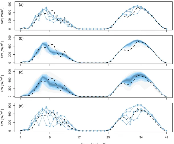
in the set defined in Eqs (2.4) can be derived for example by interpolation (Hyndman and Fan, 1996). Figure 2.2(a) shows an example of COSMO-DE-EPS global radiation forecasts and the correspond-ing station measurements. This example covers 2 consecutive days and illustrates the typical diurnal cycle associated with this weather variable. In Figure 2.2(b), the ensemble is interpreted in terms of quantile forecasts as a function of the forecast horizon. Quantiles are provided at probability levels ranging between 10% and 90% with a 10% interval. The verification of these probabilistic products is discussed in the next chapter. A subjective assessment already suggests that the ensemble variability is not able to fully capture the observation variability. Appropriate techniques can correct for this type of ensemble drawback in order to providecalibratedquantile forecasts and to generateconsistent

scenarios as shown in Figure 2.2(c) and (d), respectively. These post-processing techniques are dis-cussed in Chapter 4.

SW [ W m 2] 0 300 600 900 (a) SW [ W m 2] 0 300 600 900 (b) SW [ W m 2] 0 300 600 900 (c) Forecast horizon [h] SW [ W m 2] 1 9 17 25 34 41 0 300 600 900 (d)

Figure 2.2: Example of ensemble forecasts, ensemble interpretation, and ensemble post-processing, based on COSMO-DE-EPS global radiation forecasts of the 03UTC run on July 9, 2015, valid at sta-tion Leipzig: (a) 5 of the 20 ensemble members, (b) the ensemble forecasts interpreted in terms of quantile forecasts at probability levels 10%, 20%, ..., 80%, 90%, (c) quantile forecasts calibrated by pe-nalized quantile regression (see Section 4.2) at the same probability levels, (d) 5 of the 20 calibrated scenarios generated with a dual ensemble copula coupling approach (see Section 4.4) associated to the 5 ensemble forecasts shown in (a). The forecasts are plotted as a function of the forecast horizon. The corresponding pyranometer measurements are represented by a black dashed line.

Using the words of Atger (2004), the verification of ensemble-based probabilistic forecasts follows two goals: the validation of the system and the evaluation of end-product performance. Here, these two aspects are investigated for global radiation forecasts from COSMO-DE-EPS. The aim is to demonstrate the benefit of the ensemble approach and to provide evidence of the ensemble forecast deficiencies. In terms of products, the ensemble performance is examined with a focus on quantile forecasts, which are relevant probabilistic products for renewable energy applications. A general framework is first defined in order to describe appropriate tools and discuss their interpretation1_.

Forecast verification is here intended as the process of analysing the joint probability distribution of the forecast and the corresponding observation, where both observation and forecast are treated as random variables (Murphy and Winkler, 1987; Murphy, 1993). Considering the observation

Y = {(y, FY(y), y ∈ R)} and the forecastX = {(x, FX(x), x ∈ R)}, the joint distribution is

de-notedFY X(y, x). The verification process consists in reducing the analysis ofFY X(y, x)to a single

dimension. Scoring rules, and more generally verification measures, try to summarise in the form of a single value some aspects of the forecast performance that necessarily implies to concurrently discard information about the joint distribution (Wilks, 2006b).

Particular aspects of the forecast performance, often referred to as forecast attributes, can be drawn from the investigation of the properties of the joint distribution (Murphy and Winkler, 1987). Follow-ing the multiplicative law of probability, two manipulations of the joint distribution can be applied for this purpose. Thecalibration-refinementfactorisation,

FY X(y, x) =FY(y|X=x)FX(x), (3.1)

conditions the observation on the forecast, whereas thelikelihood-base ratefactorisation,

FY X(y, x) =FX(x|Y =y)FY(y), (3.2)

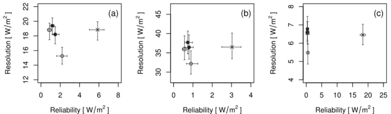
conditions the forecast on the observation. From these two factorisations, one can estimate attributes of the forecast performance such asreliability,resolution, anddiscrimination.

Adequate scores and validation tools have been developed for the verification of probabilistic pro-ducts in the form of a predictive probability distribution, a probability forecast or a quantile forecast. The decomposition of scores based on the calibration refinement factorisation provides a framework for a detailled interpretation of the results in terms of forecast statistical inconsistency and forecast information content, which are the two fundamental aspects of the forecast performance. Based on the likelihood-base rate factorisation, the information content can be further related to the forecast value, which reflects the point of view of the user on the forecast performance (Chenet al., 1987;

3.1. PROPER SCORING RULES

Buizza, 2001). Finally, relationships between forecast value and scoring rules complete the verifica-tion picture (Murphy, 1969; Richardson, 2011). Thereby, the forecast ability to capture and resolve the observations can be assessed in a cascading process from the general to the specific forecast skill.

3.1 Proper scoring rules

Scoring rules are mathematical tools dedicated to the evaluation of probabilistic forecasts. A scoring rule measures the accuracy of a probabilistic prediction assigning a numerical score as a function of the predictive distribution and the event that materialised (Gneiting and Raftery, 2007). Historically, the Brier score is the first scoring rule that has been proposed in the context of probabilistic verifica-tion (Brier, 1950). Today, this verificaverifica-tion measure is commonly used for the assessment of a forecast expressed in terms of a probability for a discrete dichotomous event.

A fundamental characteristic of a score is itspropriety(Bröcker and Smith, 2007). A scoring function is called strictly proper when’its expectation is optimal if and only if the forecast probability represents the true distribution of the target’(Bröcker, 2009). In other words, a forecaster optimises the expected score by issuing his truth believes, avoiding therefore hedging (Murphy and Epstein, 1967). For example, propriety is a characteristic of the Brier score (Murphy, 1973).

In order to provide a formal definition of a proper score, let’s notesa score of a probabilistic forecast P ∈ P and the corresponding observationω ∈ Ω. The score sis in the following considered as negatively oriented (the smaller the better) and can therefore be intended as a cost function, which is aimed to be minimized (Bentzien and Friederichs, 2014). Determined by the joint distribution

F(ω, P), the expected overall score is:

S= Z P Z Ω s(ω, P)F(ω, P)dωdP (3.3)

Applying the calibration-refinement factorisation following Eq. (3.1), the score is written as follows:

S= Z P Z Ω s(ω, P)F(ω|P)F(P)dωdP (3.4)

DenotingQ(ω) =F(ω|P)the expected distribution ofωfor a fixed probabilistic forecastP, Eq. (3.4)

is developed as: S= Z P Z Ω s(ω, P)Q(ω)F(P)dωdP = Z P S(Q, P)F(P)dP (3.5) where S(Q, P) = Z Ω s(ω, P)Q(ω)dω (3.6)

is the expected score given a forecastP. By definition (Gneiting and Raftery, 2007), the score function Sis proper if:

S(Q, Q)≤S(Q, P) (3.7)

for allP. It is strictly proper if equality is given if and only ifP =Q.

Proper scoring rules also include the Quantile Score (QS), the natural score for the assessment of quantile forecasts (Koenker and Bassett, 1978; Friederichs and Hense, 2007; Bentzien and Friederichs, 2014). QS is based on an asymmetric piecewise linear function called check function and noted

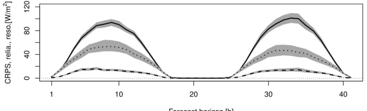
0 40 80 120 Forecast horizon [h] CRPS , relia., reso .[W/ m 2 ] 1 10 20 30 40

Figure 3.1: CRPS (full line), CRPS reliability (dashed line), and resolution components (dotted line) as a function of the forecast horizon. The confidence intervals are estimated by block bootstrapping. Results for the period July-August 2015.

ρ. Considering the pairs of quantile forecastsqτ,i at probability levelτ and observationsyi of the

verification sample withi∈1, ..., N, QS is defined as:

QSτ = 1 N N X i=1 ρτ(yi−qτ,i) (3.8) with ρτ(u) = τ u if u≥0 (τ −1)u if u <0. (3.9)

The asymmetry of the loss function is related to the probability level of the quantile forecast under assessment. Both are defined byτ which makes the link between user and probabilistic product

ex-plicit.

Each ensemble member can be interpreted as a quantile considering its rank within the ensemble sample (see Section 2.2). Therefore, the assessment of an ensemble forecast as a whole can consist in applying QS to each quantile defined by the ensemble size. This approach leads to the estimation of the continuous ranked probability score (CRPS), which is a common proper scoring rule for the verification of predictive density functions (Matheson and Winkler, 1976; Bouttier, 1994; Hersbach, 2000; Gneiting and Raftery, 2007). In the ensemble case, the CRPS follows:

CRPS= 2 M M X m=1 QSτm (3.10)

whereM is the ensemble size andτm the probability level defined in Eq. (2.4) (Bröcker, 2012). In

the continuous case, the CRPS corresponds to the integral of QS over all probability levels or equi-valently to the integral of the Brier score over all possible thresholds.

In Figure 3.1, the performance of COSMO-DE-EPS global radiation forecasts is estimated in terms of CRPS. The verification results summarize thequalityof the forecast considering all types of events and users. Plotted as a function of the forecast horizon, the score is strongly influenced by the diurnal cycle. However, it appears that the forecast exhibits a larger error in day 2 with respect to day 1. A deeper insight in the forecast performance is provided with the help of a score decomposition based on the calibration-refinement factorisation.

3.2. SCORE DECOMPOSITION

3.2 Score decomposition

The decomposition of a score in terms of reliability, resolution and uncertainty has been first pro-posed for the Brier score (Murphy, 1973; Murphy and Winkler, 1987). This decomposition becomes a standard tool for the interpretation of verification results based on this score. Moreover, a finer analysis of the reliability component can be performed based on a related graphical tool: the reliabil-ity diagram. The statistical consistency between forecast probability and observed binary outcomes is represented plotting the relative frequency of observed binary events as a function of the forecast probability class.

Not only can the score decomposition be applied to the Brier score, but also to any proper scoring rule (De Groot and Fienberg, 1982; Bröcker, 2009). For a more detailled description of the decompo-sition procedure, the terms ofentropyanddivergenceare first defined (Gneiting and Raftery, 2007). The entropy corresponds to the minimum achievable score considering the set of observationsΩ. Following Eq. (3.7), the entropy is noted as follows:

e(Q) =S(Q, Q). (3.11)

The divergence is defined as the difference between the expected score and the entropy:

d(P, Q) =S(P, Q)−S(Q, Q). (3.12)

The divergence of a negatively oriented proper score is by definition non negative (see again Eq. 3.7), and is commonly referred to as thereliabilityterm. Reliability measures the statistical consistency (or more exactly here the statistical divergence) of the forecastP with respect to the distributionQ, which

is the expected distribution of the observation givenP. The reliability term is negatively oriented (the

lower the better).

Introducing a climatological forecast_Q¯_{, estimated as the marginal distribution of the observations,} the entropy can be further decomposed:

e(Q) =S( ¯Q, Q)−d( ¯Q, Q) (3.13) whereS( ¯Q, Q)is the expected score of the climatological forecast, andd( ¯Q, Q)is the divergence be-tween the forecast and the climatological forecast. The first term is referred to asuncertaintyand is a function of the observation only. The second term, calledresolution, is related to the discrimi-nation ability of the distributionQunder different forecastP and thus is a measure of the forecast

information content (DelSole, 2004). The resolution term is positively oriented (the higher, the better). A proper scoreScan be finally decomposed as follows:

S(P, Q) =d(P, Q)−d( ¯Q, Q) +S( ¯Q,Q¯) (3.14) where the three terms on the right side of the equation are the reliability, resolution, and uncertainty terms, respectively. Integrating over all possible forecastsP, the 3 components of the overall score

are estimated.

Recently, it has been proposed a decomposition of the quantile score which participates to the ef-fort of providing equivalent tools for the verification of quantile forecasts as for the verification of probability forecasts (Bentzien and Friederichs, 2014). Formally, the decomposition of QS is noted:

QSτ =QSτreliability−QSτresolution+QSτuncertainty (3.15)

where QSreliabilityτ ,QSτresolution, andQS

uncertainty

τ are the reliability, resolution, and uncertainty terms of

the quantile score at probability levelτ, respectively. Similarly as in the categorical case, a

graph-ical tool called quantile reliability diagram provides a representation of the forecast reliability per-formance. Conditional quantiles of the observations are plotted as a function of quantile forecast

classes. A deviation of the reliability curve from the diagonal is interpreted as a lack of reliability. The decomposition of the CRPS can directly be derived from the decomposition of QS described in Eq. (3.15). Based on the definition of the CRPS in terms of QS in Eq. (3.10), a natural decomposition of CRPS in the ensemble case follows:

CRP S= 2 M M X m=1 QSτreliabilitym − 2 M M X m=1 QSτresolutionm + 2 M M X m=1 QSτuncertaintym (3.16)

where the three terms on the right of the equation are the CRPS reliability, resolution, and uncer-tainty terms, respectively. In the continuous case the weighted sum is replaced by the integral over all probability levels. Similarly, the CRPS decomposition can be based on the integration of the Brier score components over all thresholds (Candille and Talagrand, 2005). This approach is however dif-ferent from the commonly used CRPS decomposition proposed by Hersbach (2000), which is based on the average interval lengths between two successive ensemble values (Tödter and Ahrens, 2012). In Figure 3.1, besides the CRPS are plotted the corresponding reliability and resolution components. The uncertainty component is not shown since it is a property of the observations only. The decom-position allows a deeper interpretation of the performance results. The decrease in forecast quality from day 1 to day 2 is mainly explained by a decrease in forecast resolution. The information content of the ensemble forecast tends to decline with the forecast horizon. The reliability term follows a di-urnal pattern similar over the two days and significantly contributes to the CRPS estimation. Thus, the ensemble suffers from statistical inconsistencies that significantly deteriorate the reliability of the ensemble forecasts.

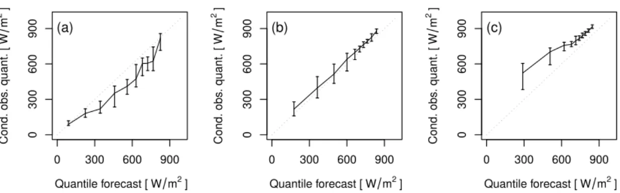
Based on QS and its decomposition, a deeper analysis of the forecast statistical properties with re-spect to the observations is performed at the product level. The graphical representation of the QS reliability component with the help of reliability diagrams evidences with more details the statistical deficiencies of the forecast. In Figure 3.2, quantile reliability diagrams are shown for quantiles at three probability levels: 10%, 50% and, 90%. Negative and positive biases affect low and high prob-ability levels, respectively, while quantile forecasts at intermediate levels are well calibrated. This configuration of quantile forecast biases is typically related to underdispersiveness in the ensemble. Moreover, the asymmetry of the biases at low and high probability levels indicates an overall nega-tive bias of the forecast. Now, a deeper analysis of the information content is discussed based on the concept of forecast value.

3.3 Quantile forecast value

The value of a forecast is examined in a risk-based decision-making framework. The estimation of whether appropriate decisions can be taken based on a forecast is directly related to the con-cept of forecast discrimination. Indeed, forecast discrimination measures the ability of a forecast to successfully discriminate between two different outcomes (Murphy, 1991). This forecast attribute is estimated based on the second factorisation of the joint probability distribution, that is the likelihood-refinement factorisation defined in Eq. (3.2). Discrimination ability is the convert of forecast resolu-tion, both depending on the forecast information content (Wilks, 2006b; Bröcker, 2014).

Discrimination of probability forecasts for binary outcomes is commonly investigated with a tool originating in signal detection theory: the Relative Operating Characteristic (ROC) curve (Mason, 1982). The ROC curve plots the relationship between two characteristics of a binary forecast, the Hit Rate (HR) and the False Alarm Rate (FAR), as a decision criterion varies. HR and FAR are derived from a contingency table that summarises the joint probability distribution of binary forecasts and observations. Binary observations result from the definition of an event while binary forecasts are

3.3. QUANTILE FORECAST VALUE Quantile forecast [W m2] Cond. obs . quant. [ W m 2 ] 0 300 600 900 0 300 600 900 (a) Quantile forecast [W m2] Cond. obs . quant. [ W m 2 ] 0 300 600 900 0 300 600 900 (b) Quantile forecast [W m2] Cond. obs . quant. [ W m 2 ] 0 300 600 900 0 300 600 900 (c)

Figure 3.2: Reliability diagrams for quantile forecasts at probability levels 10% (a), 50% (b), and 90% (c). The confidence intervals are estimated by block bootstrapping. Results for the period July-August 2015 and a forecast horizon of 9 hours.

here derived from continuous forecasts applying adecision criterion. The area under the ROC curve has been popularised as a summary measure of the forecast discrimination ability when the focus in on a specific event2_.

In Appendix A, an equivalent tool is proposed for the estimation of the forecast discrimination abi-lity focusing on a specific user. The so-called Relative User Characteristic (RUC) curve plots FAR and HR as the event of interest varies and the decision criteria are adjusted according to the level of risk accepted by the user (Section A.4). Indeed, the decision criteria applied to a forecast can be adjusted as a function of the sensitivity of the user to over- and under-forecasting characterised by an asymmetry levelτ. Thus, the RUC framework allows scanning the ability of a specific user to take opportune actions based on the forecast for a range of events.

The RUC framework is appropriate to the analysis of forecasts expressed in terms of a quantile since the associated probability level defined exactly the user’s risk adversity. A RUC analysis can as well be applied to a continuous deterministic forecast though this forecast is not targeteda prioriat a spe-cific user. A fair comparison between deterministic and ensemble-derived forecasts can take place in this framework: the full information from continuous forecasts can be assessed in both cases. In the following, the ensemble approach is compared to asingle runapproach, which consists in using as decision variable a single forecast randomly chosen among the 20 ensemble members.

The value of a forecast in a dichotomous decision framework can be derived from the ROC or RUC curve. For this purpose, a decision-making framework is depicted by a simple static cost-loss model (Thompson, 1962; Katz and Murphy, 1997). This model describes a situation of dichotomous deci-sions: a user has to decide whether or not to take protective action against potential occurrence of an event. The user’s decision is based on adecision variable,i.e. a forecast. Taking action implies a costCwhile a lossLis encountered when the event occurs without preventive action. The cost-loss

ratioC/L, denotedα, fully characterised the users. This model generalized to the continuous case considering an asymmetric loss functionρτ withτ = 1−α(see Eq. A.19).

Therelative value(oreconomic value)V of a forecast is estimated based on this model (Richardson,

2000; Wilks, 2001; Zhuet al., 2002). V is expressed as the reduction of mean expense when using

2 _{It has been shown that the ROC area is a particular case of the generalised discrimination score (also known as}

two-alternative forced choice test), which provides a general measure of the potential usefulness of a forecast (Mason and Weigel, 2009).

a forecast instead of climatological information relative to the case of using a perfect deterministic forecast:

V = E¯_¯climate−E¯forecast

Eclimate−E¯perfect, (3.17)

where_E¯_forecast,E¯_{perfect, andE}¯_{climate, are the mean expenses when a user takes decisions based on a} forecast, on a perfect deterministic forecast, and on climatological information, respectively. Eq. (3.17) can be developed (see Appendix A) andV noted as a function of the user’s cost-lost ratioα, the event

climatological frequency of occurrenceπand the two forecast characteristics HR and FAR:

V =        (1−FAR)− π 1−π 1−α α (1−HR) if α < π HR− 1−π π α 1−α FAR if α≥π. (3.18)

Therefore, the value estimates the relative performance of a forecast focusing on a specific event, characterised by a frequency of occurrenceπ, and simultaneously focusing on a specific user with a risk aversion defined by a cost-loss ratioα.

In Eq. (3.18), FAR and HR can be computed considering that the decision criterion applied to the forecast corresponds to the threshold applied to define the event of interest. In this case, the forecast is said to be taken atface value. If the decision criterion is optimised for the considered event/user situation,V is calledpotential value, that is, the maximum achievable value considering the forecast

at hand. Value and potential value are identical if the forecast is reliable, thus conditioned on cali-bration (Richardson, 2011). In other words, reliability is a necessary condition for the optimisation of forecast-based decision processes.

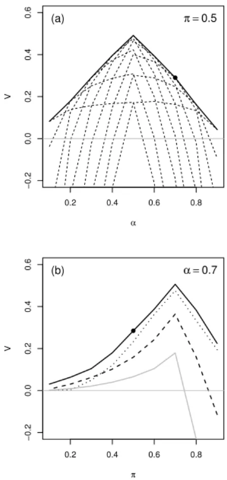
Two options have been proposed for the graphical representation of the forecast relative value, de-pending on whether the focus is on a specific event or a specific risk level. Theprobability value plot

shows the relative value of a forecast for a given event of interest as a function of the user’s cost-loss ratio. Alternatively, thequantile value plotshows the relative value of a forecast for a given cost-loss ratio as a function of the event of interest. A third option, not explored yet, would consist in sum-marising the potential value in a contour-plot with respect to the plane defined by the user’s cost-loss ratio and the event of interest.

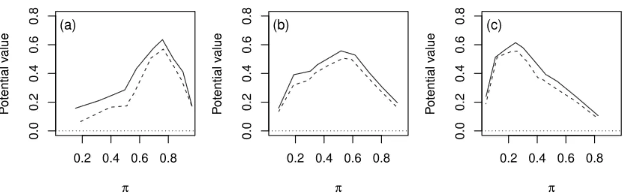
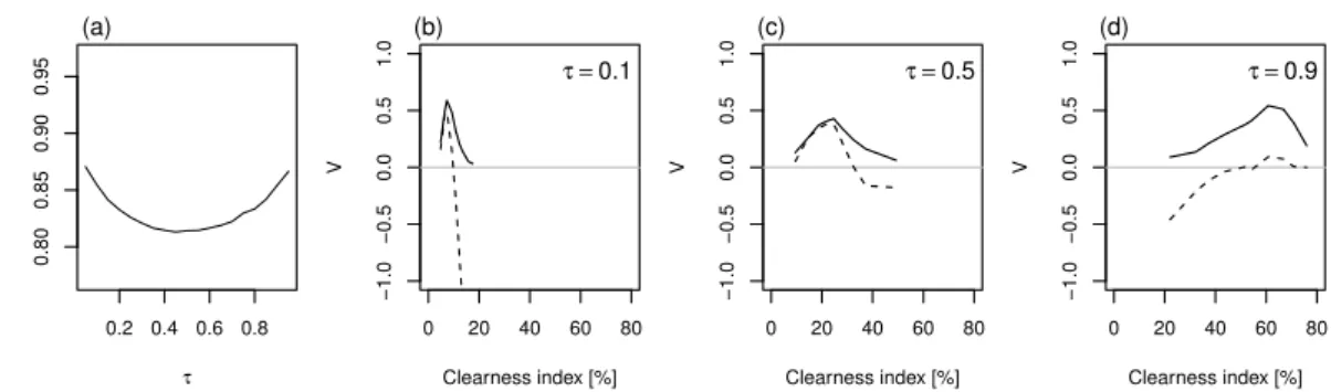
Figure 3.3 shows quantile value plots of COSMO-DE-EPS global radiation forecasts focusing on three probability levels, 25%, 50%, and 75%, corresponding to users with cost-lost ratio 75%, 50%, and 25%, respectively. More specifically, the plots represent the potential value,i.e. the value of the forecast conditioned on calibration, for forecasts valid at 12 UTC. By definition, the potential value is posi-tive and the curve reaches its maximum for events with a frequency of occurrenceπcorresponding

to1−τ. Here, the ensemble-derived forecasts are compared to deterministic forecasts. The results

show that the ensemble system outperforms the single forecast approach for the three quantile fore-casts and the whole range of events of interest investigated. So, the ensemble provides additional information with respect to deterministic forecasts and the ensemble-derived products appear to be valuable for a wide range of applications.

3.4 Ensemble added value

Relative measure of forecast performance are traditionally estimated by means ofskill scores(Wilks, 2006b). Based on negatively oriented scoring rules, skill scores have the form of a relative difference.

3.4. ENSEMBLE ADDED VALUE 0.2 0.4 0.6 0.8 0.0 0.2 0.4 0.6 0.8 π P otential v alue (a) 0.2 0.4 0.6 0.8 0.0 0.2 0.4 0.6 0.8 π P otential v alue (b) 0.2 0.4 0.6 0.8 0.0 0.2 0.4 0.6 0.8 π P otential v alue (c)

Figure 3.3: Quantile value plots showing the potential value of COSMO-DE-EPS global radiation quantile forecasts as a function of the event of interest expressed in terms of their climatological frequency of occurrence (π). Potential value of the ensemble forecast (full lines) and of a deterministic

forecast (dashed lines) for users with cost-loss ratios of 75% (a), 50% (b), and 25% (c). Results for the period July-August 2015 and a forecast horizon of 9 hours.

For example, the continuous ranked probability skill score (CRPSS) is defined as:

CRPSS= CRPS−CRPS ? CRPS−CRPS? = CRPS?−CRPS CRPS? = 1− CRPS CRPS? (3.19)

where CRPS, CRPS?_{and CRPSare the scores of the forecast under assessment, of a reference forecast}

and of a perfect deterministic forecast, respectively. The choice of the reference forecast corresponds to the goal of the comparison. Climatological forecasts or persistence forecasts are chosen as refe-rence in order to show the benefit of a forecasting system with respect to a cost-free approach. Skill scores help also to demonstrate the improvement reached by a new numerical model with respect to an older version or to compare two concurrent systems.

Here, the performance of the ensemble forecast is compared to a single forecast. The deterministic forecast is used as benchmark in order to focus on the intrinsic benefit of the computationally expen-sive ensemble system. A difficulty arises since the two forecasting approaches are by nature different: the first one is probabilistic while the second one is deterministic. Since the CRPS reduces to the Mean Absolute Error (MAE) in the single forecast case, a simple approach could consist in comparing the CRPS of the ensemble forecast and the MAE of a single run. By doing so, the comparison confronts a probabilistic interpretation of a probabilistic forecast on one side, and a deterministic interpretation of a deterministic forecast on the other side. For a fair comparison, both types of forecasts should be interpreted in a probabilistic framework.

For this purpose, consider stochastic optimisation based on a single or an ensemble forecast. In a risk-based decision-making framework, the decision criterion applied to a forecast is adjusted as a function of the user’s cost-loss ratio. This can be done independently of the nature of the forecast. Therefore, the results of decisions based on an ensemble-derived forecast or a deterministic forecast can be compared in a fair manner. This approach has been followed for the comparison of quantile forecasts and single run forecasts in terms of potential value as shown in Figure 3.3. Furthermore, the comparison can be extended to more than one single user and one single event using the relation-ships between relative value and proper scoring rules. Indeed, integrating the forecast value over all cost-loss ratios or over all events leads to the definition of the Brier skill score and quantile skill score, respectively (Murphy, 1969, Section A.6).

The potential value of a forecast is by definition estimated conditioned on calibration. Similarly, per-formance measures can focus on the information content only. Practically, it consists in considering the entropy of a scoring rule, the minimum achievable score for a given dataset. The integration of the score entropy as defined in Eq. (3.11) over all forecasts leads to the concept ofpotentialscore. The potential CRPS is defined as the difference between the uncertainty and resolution components, thus: CRPSpotential= 2 M M X m=1 (QSuncertainty τm −QS resolution τm ) (3.20)

where QSuncertaintyτm and QS resolution

τm are the uncertainty and resolution components of the QS at proba-bility levelτm, respectively. Their difference corresponds to the potential QS, the potential value of a

forecast for a given user over all thresholds.

Introduced in Appendix B, theensemble added value(EAV) is proposed as a new measure that sum-marises the benefit of using an ensemble forecasting system rather than a single run. EAV focuses exclusively on the information content: the forecast variability that allows taking adequate decisions is rewarded while the reliability deficiencies are seen as a decision criteria adjustment problem. The ensemble added value is expressed in the form of a skill score as:

EAV= 1−CRPS_CRPSpotential?

potential (3.21)

where CRPSpotential and CRPS?potential are the scores estimated applying Eq.(3.20) to the

ensemble-derived quantile forecasts and to the reference deterministic forecast, respectively.

In Figure 3.4, EAV of COSMO-DE-EPS global radiation forecasts is plotted as a function of the fore-cast horizon. One forefore-cast is chosen randomly among the 20 ensemble members for each verification day and designated as reference deterministic forecast. The relative potential benefit of the ensemble approach ranges between 5% and 15% and tends to increase with the forecast horizon. Indeed, the benefit over day 2 appears to be higher than over day 1. Despite the decrease in resolution with the forecast horizon noted in Figure 3.1, the resolution of the deterministic forecast tends to zero at a faster rate than the resolution of the probabilistic forecast. In other words, the information content in the ensemble increases with respect to the information content in the single run case, so the use of ensemble forecasts is particularly valuable for long lead times.

The potential benefit of COSMO-DE-EPS global radiation forecasts shown in Figure 3.4 as well as the economic value presented in Figure 3.3 are conditioned on calibration. However, the ensemble sys-tem demonstrates not to provide reliable probabilistic forecasts in all cases. COSMO-DE-EPS global radiation forecasts suffer from statistical inconsistencies,i.e. biases and ensemble underdispersive-ness. The lack of reliability varies as a function of the forecast horizon (see Figure 3.1), of the risk level associated with a probabilistic product (Figure 3.2), and also of the time of the year (see AppendixB). Now, these deficiencies have to be corrected by adequate methods in order to fully benefit from the ensemble approach.

3.4. ENSEMBLE ADDED VALUE Forecast horizon [h] EA V 1 10 20 30 40 0 0.1 0.2

Figure 3.4: Ensemble added value of the global radiation forecasts derived from COSMO-DE-EPS with respect to a single member approach as a function of the forecast horizon. The confidence intervals are estimated by block bootstrapping. Results for the period July-August 2015.

Post-processing is a fundamental step in the whole process of providing the users with reliable pro-babilistic forecasts based on ensemble simulations. Reliability is a necessary condition for the optimi-sation of a decision-making process (see Chapter 3). However, ensemble global radiation forecasts, and more generally ensemble forecasts of surface variables, suffer from biases and spread deficit that affect the reliability of the derived probabilistic products. Adequate calibration techniques that cor-rect for these drawbacks are therefore required.

Based on historical data, statistical post-processing consists in the application of learning algorithms aiming at the correction of systematic forecast deficiencies. Historically, post-processing of ensemble forecasts has first been tackled as a probability bias problem that can be solved with a reassignment of the probability forecasts (Murphy, 1993; Atger, 2004). For example, considering that the frequency of an observed event is, say 25%, for all cases where a system issues a probability forecast of, say 20%, a non-parametric calibration technique consists in assigning the probability 25% when the probability forecast is 20%. Using such an approach for all probability classes, the statistical discrepancy of the probability forecast is corrected and the forecast is said to be reliable. Since the forecast information content is not modified with this simple readjustment, forecast resolution and discrimination ability are not affected by calibration in that case1_.

Numerous ensemble calibration methods have been developed in recent years for a wide range of applications (Gneitinget al., 2005; Wilks, 2006a; Wilks and Hamill, 2007). On the one hand, semi-parametric approaches focus on derived probabilities or on derived quantiles, such as logistic regres-sion (Hamillet al., 2004; 2007) or quantile regression (Bentzien and Friederichs, 2012), respectively. On the other hand, fully parametric approaches are based on the definition of predictive distribu-tions as a whole and require to apply distribution fit (Gneitinget al., 2005), kernel dressing (Bröcker and Smith, 2008) or Bayesian model averaging (Rafteryet al., 2005). The frontiers between the dif-ferent approaches are however often porous. For example, logistic regression can be generalized to a distributive approach by means of an extension of the regression equations, which provides a full description of the predictive distribution (Wilks, 2009; Ben Bouallègue, 2013; Messneret al., 2014b). Today, enhanced techniques are investigated that aim to benefit from the post-processing step in order to increase the discrimination ability of the forecast by correcting biases as a function of the forecast weather conditions (Wahl, 2015).

Calibration methods however usually focus only on a single or few aspects of the ensemble forecast, such as solar radiation at a given location and forecast horizon. The dependence structures of the en-semble forecast across time, space and variables are lost after the statistical adjustment performed for each marginal predictive distribution separately, whereas the variability of the forecast, both its pre-dictable and uncertainty components, is correlated in time, space and between variables. Moreover,

1 _{for this reason, it has often been argued that only the reliability (and not the resolution) of a forecast can be improved by}

4.1. MARGINAL CALIBRATION

the user’s requirements presumably cover a variety of spatial and temporal scales, or a combination of parameters of interest. For example, applications based on global radiation forecasts may focus on intraday variability or may deal with the daily mean of day-ahead forecasts, at local, regional or national scale. Global radiation forecasts are also combined with forecasts of other weather variables such as temperature at ground in order to feed a physical PV power model, or as wind in order to manage intermittent renewable sources as a whole.

The calibration of the multivariate aspect of the forecast in a single step using parametric approaches is computationally expensive and therefore not adapted to the full dimensionality of NWP forecasts (Keuneet al., 2014; Feldmannet al., 2015). Alternatively, the generation of marginal predictive distri-butions and forecast dependencies can be treated sequentially applying the famous Sklar’s theorem, which stipulates that a multivariate joint distribution can be described by its univariate marginals plus copula (Sklar, 1959). In particular, dependencies can be modelled based on information in the original ensemble forecast using empirical copula approaches that are computationally efficient. In this framework, ensemble post-processing is approached as a two-step procedure. First, the marginal calibration adjusts the predictive distributions at each forecast horizon and location. Se-cond, scenarios are generated based on the dependence structures of the original ensemble forecasts. As a result, at the end of the post-processing steps, calibrated scenarios with consistent dependence structures can be delivered to the users.

4.1 Marginal calibration

Learning algorithms applied to ensemble forecasts have the primary goal of correcting predictive distributions for their non conformity with statistical properties of the observations. This first post-processing step, called here marginal calibration, aims to generate reliable predictive marginal dis-tributions or functional of them focusing on probability forecasts or quantile forecasts at the station level. The choice of the calibration method depends mainly on the weather parameter under focus and the end-product of interest (Hagedornet al., 2007; Hamillet al., 2007; Messneret al., 2014a). The aim here is to provide probabilistic forecasts of global radiation in terms of quantiles in order to feed an empirical copula model in a second post-processing step (see Sections 4.3 and 4.4).

Ensemble calibration has been investigated intensively for weather variables such as temperature, precipitation, or wind, but only recently applied to global radiation forecasts (e.g. Wilks and Hamill, 2007; Junket al., 2014; Zamoet al., 2014b). In Appendix C, quantile regression (QR) demonstrates to be an appropriate technique for the calibration of ensemble global radiation forecasts. Conveniently, quantile forecasts at nominal probability levels of interest are directly calibrated without assump-tions about the form of the underlying probability distribution. Moreover, QR can be indifferently applied to a probabilistic or a deterministic forecast. In the following, this characteristic of the cali-bration method allows to develop the comparison of probabilistic products derived from ensemble and single forecasts initiated in Chapter 3.

QR is a regression technique proposed by Koenker and Bassett (1978). Applied to the response vari-ableY, QR estimates quantilesQτ of the variable distributionFY(y)conditional on a set of predictors

based on a linear model. Considering a sample of observations{y1, ..., yN0}withN0the size of the

training sample and a probability level of interestτ, the optimisation process consists in minimising

asymmetrically weighted absolute residuals:

min θ∈R N0 X j=1 ρτ(yj−θ) (4.1)

whereρτ is the check function, the asymmetric loss function defined in Eq. (3.9). Replacing the scalar θby a parametric linear function, the minimisation problem is written as follows:

arg min (β0 τ,βτ) N0 X j=1 ρτ(yj−βτ0−βτvj) (4.2) whereβ0

τ andβτ are the so-called regression coefficients and{v1, ...,vN0}the vectors of predictors.

Quantile functions are estimated in the following for the probability levelsτmdefined by the

ensem-ble size following Eq. (2.4). Conditioned on the current forecastv0, the derived predictive quantile

function corresponds to:

ˆ

Qτ(y|v0) = ˆβτ0+βˆτv0 (4.3)

where the regression coefficients are estimated separately for each forecast horizon and applied in-discriminately to all locations or model grid points in this study.

The predictors that feed the regression model are usually the variables to be calibrated. For global radiation, astandard predictorsetup includes three components: the global radiation forecast itself (g),

a power transformation of the global radiation forecast (g2_{) in order to account for non-linearities,}

and the radiation at the top of the atmosphere in order to capture the natural cycle associated with the solar geometry. Applied to ensemble forecasts, the main predictorg is the first guess quantile

such asg=x(m)_wherex(m)_{is the ensemble member interpreted as a quantile forecast at probability}

levelτ =τm(Eq. 2.3). QR can also be applied to a deterministic forecast. In that case, the predictorg

corresponds to the single global radiation forecast for all examined probability levels.

Another important aspect of the first post-processing step is the definition of the historical dataset on which the optimisation process is based. Today, a standard approach consists in using a rolling window covering 4 to 10 weeks preceding the forecast to be calibrated (Gneitinget al., 2005). The dataset is updated regularly in order to follow the seasonal pattern of the forecast-observation sta-tistical characteristics. This approach has the advantage of being appropriate for operational suites with frequent updates of the underlying model. The training dataset is here defined as a rolling win-dow of 45 days updated on a daily basis.

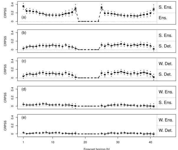
With this setup, QR is applied to COSMO-DE-EPS global radiation forecasts and the impact of cali-bration on the forecast performance is assessed over a 2 month period. Verification results are sum-marised by means of the CRPSS. In Figure 4.1(a), calibrated ensemble forecasts are compared to raw ensemble forecasts showing a significant increase of the forecast performance after calibration for all daytime forecast horizons. Ranging between 15% and 40%, the improvement is more important for sunrise/sunset hours but almost similar for day 1 and day 2. A deeper analysis is based on the CRPS and QS decompositions (not shown). The decomposition of the CRPS applied to the calibrated forecasts indicates that the reliability component becomes negligible and the resolution component remains unaffected after the calibration step. Moreover, at the product level, the inspection of quan-tile reliability diagrams demonstrates that the standard calibration approach is effective in providing reliable probabilistic products.

In a second experiment, probabilistic forecasts are this time derived from deterministic forecasts us-ing the same statistical method (QR) and a trainus-ing sample of the same size (45 days). The derived calibrated quantile forecasts, based on a single run approach, are used as reference forecasts for the computation of the CRPSS in Figure 4.1(b). Calibrated forecasts appear to be significantly better when derived from the ensemble forecasts rather than from single runs. The forecasts are reliable in both cases as checked by reliability diagrams (not shown). The performance difference lies in the higher information content in the ensemble case compared to the purely statistical approach. The re-sult of this comparison was expected: CRPSS in Figure 4.1(b) and EAV in Figure 3.4 are the practical

4.2. WEATHER-DEPENDENT CALIBRATION CRPSS (a) 0 0.2 0.4 S. Ens. Ens. CRPSS (b) 0 0.2 0.4 S. Ens