Data and Computation Efficient Meta-Learning

Meta-Learning

John Fitzgerald Bronskill

University of Cambridge

This thesis is submitted for the degree of Doctor of Philosophy

This thesis is the result of my own work and includes nothing which is the outcome of work done in collaboration except as declared in the Preface and specified in the text. It is not substantially the same as any that I have submitted, or, is being concurrently submitted for a degree or diploma or other qualification at the University of Cambridge or any other University or similar institution except as declared in the Preface and specified in the text. I further state that no substantial part of my thesis has already been submitted, or, is being concurrently submitted for any such degree, diploma or other qualification at the University of Cambridge or any other University or similar institution except as declared in the Preface and specified in the text. It does not exceed the prescribed word limit for the relevant Degree Committee.

John Fitzgerald Bronskill July 2020

John Fitzgerald Bronskill

Abstract

In order to make predictions with high accuracy, conventional deep learning systems require large training datasets consisting of thousands or millions of examples and long training times measured in hours or days, consuming high levels of electricity with a negative impact on our environment. It is desirable to have have machine learning systems that can emulate human behavior such that they can quickly learn new concepts from only a few examples. This is especially true if we need to quickly customize or personalize machine learning models to specific scenarios where it would be impractical to acquire a large amount of training data and where a mobile device is the means for computation. We define adata efficientmachine learning system to be one that can learn a new concept from only a few examples (orshots) and acomputation efficientmachine learning system to be one that can learn a new concept rapidly without retraining on an everyday computing device such as a smart phone.

In this work, we design, develop, analyze, and extend the theory of machine learning systems that are bothdata efficientandcomputation efficient. We present systems that are trained using multiple tasks such that it "learns how to learn" to solve new tasks from only a few examples. These systems can efficiently solve new, unseen tasks drawn from a broad range of data distributions, in both the low and high data regimes, without the need for costly retraining. Adapting to a new task requires only a forward pass of the example task data through the trained network making the learning of new tasks possible on mobile devices. In particular, we focus on few-shot image classification systems, i.e. machine learning systems that can distinguish between numerous classes of objects depicted in digital images given only a few examples of each class of object to learn from.

To accomplish this, we first develop ML-PIP, a general framework for Meta-Learning approximate Probabilistic Inference for Prediction. ML-PIP extends existing probabilistic interpretations of meta-learning to cover a broad class of methods. We then introduce VERSA, an instance of the framework employing a fast, flexible and versatile amortization network that takes few-shot learning datasets as inputs, with arbitrary numbers of training examples, and outputs a distribution over task-specific parameters in a single forward pass of the network. We evaluate VERSAon benchmark datasets, where at the time, the method achieved state-of-the-art results when compared to meta-learning approaches using similar training regimes and feature extractor capacity.

Next, we build on VERSAand add a second amortized network to adapt key parameters in the feature extractor to the current task. To accomplish this, we introduce CNAPS, a conditional neural process based approach to multi-task classification. We demonstrate that, at the time, CNAPS achieved state-of-the-art results on the challenging META-DATASET

benchmark indicating high-quality transfer-learning. Timing experiments reveal that CNAPS is computationally efficient when adapting to an unseen task as it does not involve gradient back propagation computations. We show that trained models are immediately deployable to continual learning and active learning where they can outperform existing approaches that do not leverage transfer learning.

Finally, we investigate the effects of different methods of batch normalization on meta-learning systems. Batch normalization has become an essential component of deep meta-learning systems as it significantly accelerates the training of neural networks by allowing the use of higher learning rates and decreasing the sensitivity to network initialization. We show that the hierarchical nature of the meta-learning setting presents several challenges that can render conventional batch normalization ineffective. We evaluate a range of approaches to batch normalization for few-shot learning scenarios, and develop a novel approach that we call TASKNORM. Experiments demonstrate that the choice of batch normalization has a dramatic effect on both classification accuracy and training time for both gradient based- and gradient-free meta-learning approaches and that TASKNORMconsistently improves performance.

I have been very fortunate to have Richard Turner and Sebastian Nowozin as PhD supervisors. Both have provided superb guidance, deep insights, and extensive contributions to my work. I want to thank Rich for taking me on as a student even though it had been more than thirty years since I completed my Masters degree. Being in Rich’s group has been a fantastic experience and a great privilege. I have always had deep respect for Sebastian’s work and know-how and I am lucky that he agreed to co-supervise and contribute numerous key ideas and suggestions. I would also like to thank my advisor Dr. José Miguel Hernández Lobato for his support.

I was also very fortunate to have a desk next to Jonathan Gordon who has been a fabulous collaborator. I learned a lot from him and he contributed jointly to almost all aspects of the research contained in this thesis. I would also like to acknowledge the valuable and significant contributions of my other awesome student collaborators and co-authors Matthias Bauer and James Requeima - it has been a great pleasure to work with both of them.

Finally, a big thanks to all the members of the Computational and Biological Learning group at the University of Cambridge for helping make my PhD experience so enjoyable.

List of figures xv

List of tables xvii

Nomenclature xix

1 Introduction 1

1.1 Motivation . . . 1

1.2 Overview and Main Contributions . . . 2

1.3 List of Publications . . . 4

1.3.1 Conference Proceedings . . . 4

1.3.2 Workshops . . . 5

1.3.3 Source Code Repositories . . . 5

2 Background 7 2.1 Meta-Learning, Multi-Task Learning, and Transfer Learning . . . 7

2.1.1 Meta-Learning . . . 7

2.1.2 Multi-Task Learning . . . 8

2.1.3 Transfer Learning . . . 9

2.2 Few-Shot Learning Fundamentals . . . 9

2.2.1 Tasks, Context and Target Sets . . . 9

2.2.2 Episodic Training . . . 10

2.2.3 Hierarchical Probabilistic Modelling View of Meta-Learning . . . 12

2.3 Meta-learning Methods . . . 14

2.3.1 Multi-step Gradient Approaches . . . 16

2.3.2 Few-step Gradient Approaches . . . 16

2.3.3 Amortization via Hypernetworks . . . 19

2.3.4 Semi-amortized Approaches . . . 23

2.3.5 Probabilistic Methods . . . 24

2.4 Neural Processes . . . 26

2.4.2 Neural Processes . . . 27

2.4.3 Generative Query Networks for View Reconstruction . . . 28

2.5 Continual Learning and Amortized Inference Methods . . . 30

2.6 Active Learning and Few-shot Learning . . . 31

2.7 Datasets for Few-Shot Classification . . . 31

2.7.1 Omniglot . . . 32

2.7.2 miniImageNet . . . 32

2.7.3 META-DATASET . . . 33

2.8 Conclusion . . . 34

3 VERSA: Meta-Learning Probabilistic Inference For Prediction 37 3.1 Introduction . . . 37

3.2 Meta-Learning Probabilistic Inference For Prediction . . . 38

3.2.1 Probabilistic Model . . . 38

3.2.2 Probabilistic Inference . . . 39

3.3 Versatile Amortized Inference . . . 42

3.4 Variational Inference Derivations for the Model . . . 45

3.5 ML-PIP Unifies Disparate Related Work . . . 45

3.6 Experiments and Results . . . 47

3.6.1 Posterior Inference with Toy Data . . . 47

3.6.2 Few-shot Classification . . . 48

3.6.3 ShapeNet View Reconstruction . . . 51

3.7 Summary . . . 54

3.8 Epilogue . . . 54

4 CNAPS: Fast and Flexible Multi-Task Classification Using Conditional Neural Adap-tive Processes 57 4.1 Introduction . . . 57

4.2 Model Design . . . 59

4.2.1 Specification of the classifier: globalθand task-specific parametersψτ . 60 4.2.2 Computing the local parameters via adaptation networks . . . 61

4.3 Model Training . . . 64

4.4 Related Work . . . 65

4.5 Experiments and Results . . . 66

4.6 Continual Learning . . . 69

4.7 Active Learning . . . 72

4.8 Summary . . . 73

5 TASKNORM: Rethinking Batch Normalization for Meta-Learning 79

5.1 Introduction . . . 79

5.2 Background and Related Work . . . 80

5.2.1 Normalization Layers in Deep Learning . . . 80

5.2.2 Desiderata for Meta-Learning Normalization Layers . . . 81

5.3 Normalization Layers for Meta-learning . . . 83

5.3.1 Conventional Usage of Batch Normalization (CBN) . . . 83

5.3.2 Batch Renormalization (BRN) . . . 83

5.3.3 Transductive Batch Normalization (TBN) . . . 84

5.3.4 Instance-Based Normalization Schemes . . . 85

5.3.5 Other NLs . . . 86

5.4 Task Normalization . . . 86

5.4.1 Meta-Batch Normalization (METABN) . . . 87

5.4.2 TASKNORM . . . 87

5.5 Experiments . . . 89

5.5.1 Small Scale Few-Shot Classification Experiments . . . 89

5.5.2 Large Scale Few-Shot Classification Experiments . . . 92

5.5.3 Transduction Tests . . . 94

5.5.4 Ablation Study: Choosing the best parameterization forα . . . 95

5.5.5 Evolution ofαas Training Progresses . . . 98

5.6 Summary . . . 98

6 Conclusions and Discussion 101 6.1 Summary . . . 101

6.1.1 Primary Contributions . . . 101

6.2 Discussion . . . 102

6.2.1 Building a State-of-the-Art Few-shot, Multi-task Image Classifier . . . . 102

6.2.2 Future Work . . . 105

References 109 Appendix A Additional Modeling Details and Experiments 121 A.1 Additional ML-PIP Modeling Details and Experiments . . . 121

A.1.1 Bayesian Decision Theoretic Generalization of ML-PIP . . . 121

A.1.2 Justification for Context-Independent Approximation . . . 123

A.2 Additional CNAPSFew-Shot Classification Results . . . 125

A.2.1 Joint Training ofθandϕ . . . 125

Appendix B Experiment Details 129

B.1 VERSAExperimentation Details . . . 129

B.1.1 Omniglot Few-shot Classification Training Procedure . . . 129

B.1.2 miniImageNET Few-shot Classification Training Procedure . . . 130

B.2 CNAPSExperimentation Details . . . 130

B.2.1 META-DATASETTraining and Evaluation Procedure . . . 130

B.2.2 Continual Learning Experimentation Details . . . 132

B.2.3 Active Learning Experimentation Details . . . 133

B.3 TASKNORMExperimentation Details . . . 134

B.3.1 MAML Experiments . . . 134

B.3.2 CNAPSExperiments . . . 134

B.3.3 Prototypical Networks Experiments . . . 135

Appendix C Network Architectures 137 C.1 VERSAFew-shot Classification Network Architectures . . . 137

C.2 VERSAView Reconstruction Network Architectures . . . 138

C.3 CNAPSNetwork Architectures . . . 138

C.3.1 ResNet18 Architecture details . . . 138

C.3.2 Adaptation Network Architecture Details . . . 138

2.1 Sample meta-learning task . . . 10

2.2 Episodic training . . . 11

2.3 Directed graphical model for multi-task learning . . . 13

2.4 Model design space . . . 14

2.5 Residual Adapters . . . 17

2.6 FiLM layer and its use in a residual network . . . 20

2.7 Prototypical Networks classification . . . 22

2.8 Neural process graphical models . . . 27

2.9 Conditional neural process computational flow . . . 27

2.10 3D model reconstruction from a set of photographs . . . 28

2.11 Meta-learning perspective of view reconstruction . . . 29

2.12 GQN concept and flow diagram . . . 29

2.13 Omniglot samples . . . 32

2.14 META-DATASETsamples . . . 34

3.1 Computational flow of VERSAfor few-shot classification . . . 43

3.2 Computational flow of VERSAfor few-shot view reconstruction . . . 44

3.3 Posterior inference with toy data experiment results . . . 48

3.4 Test accuracy on Omniglot when varying way and shot . . . 51

3.5 Results for ShapeNet view reconstruction for unseen objects . . . 53

4.1 Probabilistic graphical model for CNP framework and computational diagram depicting the CNAPSmodel . . . 59

4.2 Implementation of the class-specific adaptation parametersψw . . . 62

4.3 Implementation of the feature-extractor . . . 63

4.4 Adaptation networkϕf . . . 63

4.5 t-SNE plots of the FiLM layer parameters at test time . . . 69

4.6 Comparing CNAPSto gradient based feature extractor adaptation . . . 69

4.7 Continual learning classification results on Split MNIST and Split CIFAR100 . . 71

4.9 Continual learning results on Split CIFAR100 . . . 76

4.10 Accuracy vs active learning iterations for held-out classes / languages . . . 77

4.11 Complete active learning results on Omniglot . . . 78

5.1 Options for batch normalization for meta-learning . . . 82

5.2 Plots ofαas a function of context set size . . . 88

5.3 Plot of accuracy vs shot for MAML . . . 91

5.4 Training curves for small scale experiments . . . 92

5.5 Training curves for large scale experiments . . . 95

5.6 Plots of validation accuracy and training loss versus training iteration . . . 99

5.7 Plots of TASKNORMparameters versus training iteration . . . 99

5.8 Plots ofαas a function of training iteration and context set size . . . 100

A.1 Visualizing the learned weights . . . 124

3.1 Accuracy results for different few-shot settings on Omniglot andminiImageNet 50

3.2 Negative Log-likelihood results on Omniglot andminiImageNet . . . 51

3.3 List of ShapeNet categories used in the view reconstruction experiments . . . . 52

3.4 View reconstruction test results . . . 54

4.1 Few-shot classification results on META-DATASET . . . 67

4.2 Few-shot classification results using models trained on ILSVRC-2012 only . . . 68

5.1 Accuracy results for different few-shot settings on Omniglot andminiImageNet using MAML . . . 89

5.2 Accuracy results for different few-shot settings on Omniglot andminiImageNet using Prototypical Networks . . . 90

5.3 Few-shot classification results on META-DATASETusing CNAPS . . . 93

5.4 Few-shot classification results on META-DATASETusing Prototypical Networks 94 5.5 Few-shot classification results when classifying one example and one class at a time . . . 96

5.6 Results ofαparameterization tests using the MAML algorithm . . . 97

5.7 Results ofαparameterization tests using the CNAPSalgorithm . . . 98

A.1 Few-shot classification results comparing joint training to two-stage training . . 126

A.2 Few-shot classification results for Parallel Residual Adapters . . . 127

B.1 Datasets used to train, validate, and test CNAPSmodels . . . 132

C.1 Feature extraction network used for Omniglot few-shot learning . . . 137

C.2 Feature extraction network used forminiImageNet few-shot learning . . . 138

C.3 Amortization network used for Omniglot andminiImageNet few-shot learning 138 C.4 Linear classifier used for Omniglot andminiImageNet few-shot learning . . . . 139

C.5 Encoder network used for ShapeNet few-shot learning . . . 139

C.6 Amortization network used for ShapeNet few-shot learning . . . 139

C.8 ResNet-18 basic block network . . . 140

C.9 ResNet-18 basic scaling block network . . . 140

C.10 ResNet-18 feature extractor network . . . 141

C.11 Set encodergnetwork . . . 141

C.12 Set encoderϕf network . . . 141

C.13 Film generator network . . . 142

C.14 Adaptation network for classifier weights . . . 142

C.15 Adaptation network for classifier bias . . . 142

Acronyms / Abbreviations

1D 1-Dimensional 2D 2-Dimensional 3D 3-Dimensional

C-VAE Conditional Variational Autoencoder CNAPS Conditional Neural Adaptive Processes CNP Conditional Neural Process

Dτ The context set for a taskτ

GPU Graphics Processing Unit GQN Generative Query Network

i.i.d. independent and identically distributed LSTM Long Short-Term Memory

MAML Model-Agnostic Meta-Learning MAP Maximum A Posteriori

ML-PIP Meta-learning Probabilistic Inference for Prediction NL Normalization Layer

NP Neural Process

SVGD Stein Variational Gradient Descent

Tτ The target set for a taskτ

Introduction

1.1

Motivation

Humans are able to learn a new concept from just a few examples and can leverage past experience with concepts in one domain to learn new concepts in a different domain (Lake et al., 2011). In addition, humans can learn continuously with minimal forgetting of older concepts. In the quest to emulate this ability, the machine learning community has made spectacular advances in the areas of computer vision (Krizhevsky et al.,2012), natural language processing (Devlin et al.,2018), and speech recognition (Xiong et al.,2018). Despite this, to learn new concepts or tasks, conventional deep learning techniques:

• require thousands of training examples (e.g. training an image classifier on ImageNet to achieve state of the art accuracy requires 1300 labeled examples per class (Krizhevsky et al.,2012));

• overfit when only a few training examples are available (Goodfellow et al.,2016); • have only basic ability for leveraging previous learning (e.g. transfer learning (Pratt et al.,

1991) or fine-tuning (Yosinski et al.,2014)) and this is typically done attrainingtime as opposed to post-trainingdeploymenttime;

• exhibit catastrophic forgetting (i.e. the tendency for a neural network to suddenly lose knowledge it had already learned when learning new information (French,1999)); • need long training times measured in hours or days, which result in high computation

costs, large power consumption and carbon dioxide emmisions. For example, training the BERT model (Devlin et al.,2018) takes 79 hours using 64 NVIDIA V100 GPUs, costing up to USD12,571 of cloud computing time, utilizing an effective 1507 kilowatt-hours of electricity (about the same as used by the average UK citizen in 15 weeks) and emitting 1438 pounds of carbon dioxide (about the same emitted by the average UK citizen over a period of 5 weeks) (Strubell et al.,2019);

• are trained offline using specialized computing platforms (e.g. cloud data center, GPU cluster, etc.) as opposed to online on common computing devices; and

• have difficulty adding new classes or datasets in the classification setting without re-training.

On the other hand, we desire machine learning systems that are:

• data efficient: able to learn a new task from only a few examples without over-fitting, but be resistant to under-fitting if more data is available;

• computation efficient: able to learn a new task rapidly without retraining on common computing platforms (e.g. on a mobile device);

• make predictions in real-time in a power efficient manner on common computing plat-forms (e.g. on a mobile device);

• share knowledge across tasks;

• learn continuously, without forgetting.

In this thesis we aim to design, develop, analyze, and extend the theory of machine learning systems that are bothdata efficientandcomputation efficient. During training, our system is exposed to multiple tasks such that it "learns how to learn" (i.e. meta-learns) to solve new tasks from only a few examples. The system can effectively and efficiently solve new, unseen tasks from a broad range of data distributions, in both the low and high data regimes, without the need for costly retraining. Adapting to a new task requires only a forward pass of the example task data through the trained network making the learning of new tasks possible on mobile devices.

In particular, we focus on few-shot image classification systems. We argue that such systems require mechanisms that adapt to each task, and that these mechanisms should themselves be learned from a diversity of datasets and tasks at training time. The adaptation mechanism should affect the entire system, not just the classifier component and the resulting system should be adept at continual learning.

1.2

Overview and Main Contributions

This section provides an overview of the work contained in this thesis. For each topic, the main results are summarized and the publications that I co-authored with my supervisors and fellow students that resulted from the research are cited. My personal contributions to each topic are listed at the beginning of the respective chapters.

VERSA: Meta-Learning Probabilistic Inference For Prediction Chapter 3introduces a new

framework for data efficient, computation efficient, and versatile learning. Specifically: (i) We develop ML-PIP, a general framework for Meta-Learning approximate Probabilistic Inference for Prediction. ML-PIP extends existing probabilistic interpretations of meta-learning to cover a broad class of methods. (ii) We introduce VERSA, an instance of the framework employing a fast, flexible and versatile amortization network that takes few-shot learning datasets as inputs, with arbitrary numbers of training examples, and outputs a distribution over task-specific parameters in a single forward pass of the network. VERSAsubstitutes optimization at test time with forward passes through inference networks, amortizing the cost of inference and relieving the need for second derivatives during training. (iii) We evaluate VERSA on benchmark datasets where the method set state-of-the-art results (at the time), handles arbitrary numbers of training examples, and for classification, arbitrary numbers of classes at train and test time. The power of the approach is then demonstrated through a challenging few-shot ShapeNet view reconstruction task.

These results are joint work with my co-first author Jonathan Gordon, as well as Matthias Bauer, Sebastian Nowozin, and Richard Turner and were published as ‘Meta-Learning Proba-bilistic Inference For Prediction’ (Gordon et al.,2019) in the ICLR 2019 conference proceedings. CNAPS: Fast and Flexible Multi-Task Classification Using Conditional Neural Adaptive Processes Chapter 4 builds on the work in the Chapter 3and adds a second amortized network to adapt key parameters in the feature extractor to the current task in addition to adapting the final layer classifier. To accomplish this, we introduce a conditional neural process based approach to the multi-task classification setting and establish connections to the meta-learning and few-shot learning literature. The resulting approach, called CNAPS, comprises a classifier whose parameters are modulated by an adaptation network that takes the current task’s dataset as input. We demonstrate that CNAPSachieved state-of-the-art results (at the time) on the challenging META-DATASETbenchmark indicating high-quality transfer-learning. We show that the approach is robust, avoiding both over-fitting in low-shot regimes and under-fitting in high-shot regimes. Timing experiments reveal that CNAPSis computationally efficient at test-time as it does not involve gradient based adaptation. Finally, we show that trained models are immediately deployable to continual learning and active learning where they can outperform existing approaches that do not leverage transfer learning.

These results are joint work with my co-first authors James Requeima and Jonathan Gordon, as well as Sebastian Nowozin, and Richard Turner and were published as ‘Fast and Flexible Multi-Task Classification Using Conditional Neural Adaptive Processes’ (Requeima et al., 2019b) in the NeurIPS 2019 conference proceedings and was selected for a spotlight talk. TASKNORM: Rethinking Batch Normalization for Meta-Learning Chapter 3 and

increasingly deep networks to achieve state-of-the-art performance, making batch normal-ization an essential component of meta-learning pipelines. However, the hierarchical nature of the meta-learning setting presents several challenges that can render conventional batch normalization ineffective, giving rise to the need to rethink normalization in this setting. In

Chapter 5, we evaluate a range of approaches to batch normalization for meta-learning

sce-narios, and develop a novel approach that we call TASKNORM. Experiments on fourteen datasets demonstrate that the choice of batch normalization has a dramatic effect on both classification accuracy and training time for both gradient based- and gradient-free meta-learning approaches. Importantly, TASKNORMis found to consistently improve performance. Finally, we provide a set of best practices for normalization that will allow fair comparison of meta-learning algorithms.

These results are joint work with my co-first author Jonathan Gordon, as well as James Requeima, Sebastian Nowozin, and Richard Turner and were published as ‘TASKNORM: Rethinking Batch Normalization for Meta-Learning’ in the ICML 2020 conference proceedings. (Bronskill et al.,2020).

1.3

List of Publications

The following provides a list of all publications I have co-authored in the course of pursuing my DPhil degree.

1.3.1 Conference Proceedings

Jonathan Gordon*, John Bronskill*, Matthias Bauer, Sebastian Nowozin, and Richard Turner (2019). ‘Meta-Learning Probabilistic Inference for Prediction’. In:Proceedings of the 7th Interna-tional Conference on Learning Representations. *equal contribution

James Requeima*, Jonathan Gordon*, John Bronskill*, Sebastian Nowozin, and Richard E. Turner (2019). ‘Fast and flexible multi-task classification using conditional neural adaptive processes.’ In: Advances in Neural Information Processing Systems 32, pages 7957–7968. This paper was selected for a spotlight presentation at the conference. *equal contribution

John Bronskill*, Jonathan Gordon*, James Requeima, Sebastian Nowozin, and Richard E. Turner (2020). ‘TASKNORM: Rethinking Batch Normalization for Meta-Learning.’ In

Proceed-ings of the 37th International Conference on Machine Learning. *equal contribution

Daniela Massiceti, John Bronskill, Luisa M. Zintgraf, Sebastian Tschiatschek, Katja Hofmann and Cecily Morrison (2020). ‘Meta-learning from Poor-Quality Videos for Personalised Object Recognition’ Submitted to:The 2020 European Conference on Computer Vision.

1.3.2 Workshops

Jonathan Gordon*, John Bronskill*, Matthias Bauer, Sebastian Nowozin and Richard E. Turner (2018). ‘Decision-Theoretic Meta-Learning: Versatile and Efficient Amortization of Few-Shot Learning’ In:International Workshop on Automatic Machine Learning (AutoML 2018) at Thirty-fifth International Conference on Machine Learning.*equal contribution

Jonathan Gordon*, John Bronskill*, Matthias Bauer*, Sebastian Nowozin, and Richard E. Turner (2018). ‘Versa: Versatile and Efficient Few-shot Learning’. In:Third Workshop on Bayesian Deep Learning at the 32nd Conference on Neural Information Processing Systems.*equal contribution

Jonathan Gordon*, John Bronskill*, Matthias Bauer*, Sebastian Nowozin, and Richard E. Turner (2018). ‘Consolidating the Meta-Learning Zoo: A Unifying Perspective as Posterior Predictive Inference’. In:Workshop on Meta-Learning (MetaLearn 2018) at the 32nd Conference on Neural Information Processing Systems.*equal contribution

1.3.3 Source Code Repositories

John Bronskill, Jonathan Gordon, and Matthias Bauer (2019). Code for ‘Meta-Learning Proba-bilistic Inference for Prediction’.https://github.com/Gordonjo/versa

John Bronskill, Jonathan Gordon, and James Requeima (2019). Code for ‘Fast and flexible multi-task classification using conditional neural adaptive processes.’ and ‘TASKNORM: Rethinking Batch Normalization for Meta-Learning.’https://github.com/cambridge-mlg/cnaps

Background

In this chapter, we review the concepts and literature that form the basis of the research work that follows. First, we give a high-level overview of Meta-Learning, Multi-Task Learning and Transfer Learning inSection 2.1. InSection 2.2, we explain the concepts that underlie few-shot learning and then inSection 2.3, we survey the few-shot learning methods that are the most relevant to the work in this thesis. InSection 2.4, we summarize Neural Processes, a meta-learning approach that combines the benefits of Gaussian Processes which are probabilistic and data efficient with the computational efficiency of deep neural networks. We then provide brief introductions to Continual Learning and Active Learning and their relationship to few-shot learning methods inSection 2.5andSection 2.6, respectively. Finally, we describe the primary datasets used to benchmark few-shot learning methods inSection 2.7.

2.1

Meta-Learning, Multi-Task Learning, and Transfer Learning

2.1.1 Meta-Learning

Conventional deep learning learning systems are normally trained to solve a specific prediction task and in doing so require copious data and computational resources (Krizhevsky et al., 2012). This can be problematic if training data or computing resources are scarce or impractical to obtain. A key concept throughout this thesis is meta-learning orlearning to learn. In meta-learning, a machine learning model gains experience over multiple learning tasks and leverages this past cross-task experience to improve future learning ability. This ability to learn how to learn leads to benefits in both data and computation efficiency (Hospedales et al.,2020).

The concept of meta-learning originated in cognitive psychology (Maudsley,1980). In computer science, early approaches to meta-learning include a system calledShift To A Better Bias(Utgoff,1986), the variable bias management system (Rendell et al.,1987) which auto-matically selects between different learning algorithms, and the work bySchmidhuber(1987) that attempts to learn entire learning algorithms via genetic evolution. Since recurrent neural networks (RNNs) are universal computers,Schmidhuber(1993) showed how self-referential RNNs can learn to run their own weight change algorithm. In this work, we focus on more recent deep learning approaches to meta-learning.

Historically, machine learning models were learned based on hand-engineered features. In the deep learning era that followed, features were jointly learned with the model. Meta-learning can be viewed as the next step in this progression by jointly Meta-learning the features, model, and the learning algorithm itself (Hospedales et al.,2020). In the context of this thesis, we use the term meta-learning to refer to the ability of a system to generate or induce a learning algorithm to meet the demands of a novel machine learning task based on experience acquired from prior tasks.

2.1.2 Multi-Task Learning

The goal of multi-task learning (Caruana,1997) is to improve learning efficiency and accuracy of prediction on a group of tasks by learning from the group of tasks in parallel, compared to training on each task separately. It accomplishes this by leveraging a shared representation between tasks i.e. what is learned for a single task will aid in the learning other tasks.Caruana (1997) shows that multi-task learning also improves generalization by leveraging the domain-specific information contained in the training signals of related tasks.

An example of this is a system to filter email that is customized for each user to only display email that is of importance to them (Edelen et al.,2019). However, some email will be important to many users, but other email will only be important for a small subset of users. When implementing such a system, one possibility is train a unique filtering model for each user in the system. Alternatively, multi-task learning could be employed to potentially improve overall accuracy across all users by leveraging various commonalities and differences across the user base. This is especially true if some email users do not receive much email and hence have little training data to contribute. Caruana(1997) shows reduction of prediction error by up to30%on certain tasks using multi-task learning versus single-task learning.

Multi-task learning differs from meta-learning in that the goal of multi-task learning is to make predictions on a fixed number of tasks whereas the goal of meta-learning is to make predictions on future tasks that are not seen during training. In addition, multi-task learning employs a single level of optimization during learning while meta-learning also employs a higher level objective to learn across many tasks such that a novel task can be rapidly solved. However, inChapter 3and Chapter 4we demonstrate that multi-task learning principles

can aid in training neural networks that learn to rapidly generate classifier parameters for classifying novel tasks.

2.1.3 Transfer Learning

Transfer learning aims to transfer knowledge from one learning task to another related task. In particular, it is common to use a source task to improve learning on a target task by transferring some or all of the parameters from the source task to the target task (Hospedales et al.,2020). For example, it is common to train a classification model on a large image dataset such as ImageNet (Russakovsky et al., 2015) and use the learned feature representations to aid classification on a different dataset such as CIFAR (Krizhevsky and Hinton,2009). This process is often referred to asfine tuningsince the transferred ImageNet features are fine-tuned with the CIFAR image data.

In an impressive success story,Bird et al.(2020) demonstrate that transfer learning between the Electroencephalographic (EEG) brainwave domain and the Electromyographic (EMG) muscular wave domain showed significant gains in classification accuracy. In particular, when the pre-trained weights from the EMG model are used to initialize training of the EEG model, classification accuracy increases to92.83%from62.37%using random initialization.

Transfer learning differs from meta-learning in that the information transferred via transfer learning is learned by conventional supervised learning on a source task without use of a higher-level meta-learning training objective that aims to learn across many tasks such that it can rapidly learn a new task. That said, inChapter 4we show how transfer learning can be used in conjunction with meta-learning to great effect by employing a pre-trained feature extractor and modulating it’s activations with meta-learned weights.

2.2

Few-Shot Learning Fundamentals

This thesis is primarily concerned with developing data and computation efficient systems for multi-task, few-shot image classification and regression based on a meta-learning approach. In this section, we describe the key ingredients for few-shot learning: task, context and target sets, as well as a meta-learning training protocol, and a probabilistic view of meta-learning.

2.2.1 Tasks, Context and Target Sets

In the following, we consider the multi-task image classification scenario. Rather than a single, large datasetD, we assume access to a datasetD = {τt}Kt=1 comprising a large number of

trainingtasksτt, drawn i.i.d. from a distributionp(τ). The data for a taskτ consists of acontext

setDτ = {(x_nτ,y_nτ)}Nτ

n=1 withNτ elements with the inputsxτn and labelsynτ observed, and a

target setTτ = {(x_mτ∗,y_mτ∗)}Mτ

m=1 withMτ elements for which we wish to make predictions.

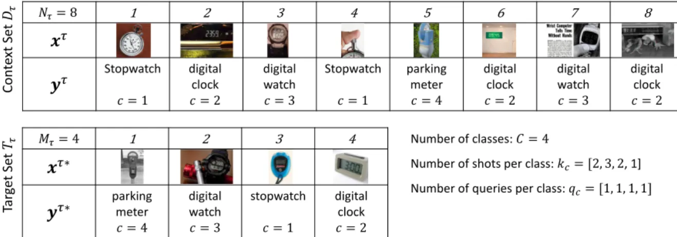
examples from a single task are assumed i.i.d., but examples across tasks are not. Note that the target set examples are drawn from the same set of labels as the examples in the context set. An example task is shown inFigure 2.1. In the few-shot learning literature, a task is also referred to as an episode. In the next section, a task-aware training regime termedepisodic

training will be described.

𝑁𝜏= 8 1 2 3 4 5 6 7 8 𝒙𝜏 𝒚𝜏 Stopwatch 𝑐 = 1 digital clock 𝑐 = 2 digital watch 𝑐 = 3 Stopwatch 𝑐 = 1 parking meter 𝑐 = 4 digital clock 𝑐 = 2 digital watch 𝑐 = 3 digital clock 𝑐 = 2 𝑀𝜏= 4 1 2 3 4 𝒙𝜏∗ 𝒚𝜏∗ parking meter 𝑐 = 4 digital watch 𝑐 = 3 stopwatch 𝑐 = 1 digital clock 𝑐 = 2 Con te xt Se t Tar ge t Se t Number of classes: 𝐶 = 4

Number of shots per class: 𝑘𝑐= [2, 3, 2, 1]

Number of queries per class:𝑞𝑐= [1, 1, 1, 1]

Fig. 2.1 A sample meta-learning task consisting of a context setDτ of sizeNτ = 8and a target

setTτ of sizeMτ = 4. Note that the labelsyτ∗would only be observed during training. The

elements of the context and target sets are drawn from four different classes - stopwatch, digital clock, digital watch, and parking meter. Another task may have different context and target sizes, different classes, a different number of classes, and different number of examples per class. Images are examples from ImageNet (Russakovsky et al.,2015).

2.2.2 Episodic Training

The majority of multi-task, few-shot classification methods that are based on meta-learning concepts use anepisodictraining and testing protocol introduced byVinyals et al.(2016). The key principle behind this protocol is that the training (referred to asmeta-training) and testing (referred to asmeta-testing) conditions should match and the system should be meta-trained with a large number of few-shot learning tasks.

The episodic training and testing protocol is described in the steps below.Figure 2.2depicts a generic meta-learning-based multi-task classification system that will be referred to in the various steps.

Meta-Training

1. Create the context and target sets. Draw a taskτ from the training datatsetDtrain as

follows.

2.2 Few-Shot Learning Fundamentals 11

Meta-learner

Classifier

Context Set

𝐷

Target

Inputs

𝒙

Classifier

Parameters

𝝍

Few-shot Learner

Loss

Function

Target

Labels

𝒚

𝑝 𝒚

𝒙

, 𝝍

)

Loss

Meta-learner

Classifier

Context Set

𝐷

Target

Inputs

𝒙

Classifier

Parameters

𝝍

Few-shot Learner

𝑝 𝒚

𝒙

, 𝝍

)

Meta-learner

Classifier

𝑓(𝒙

, 𝜽, 𝝍

)

Context Set

𝐷

Target

Inputs

𝒙

Classifier

Parameters

𝝍

Few-shot Learner

Loss

Function

ℒ

Target

Labels

𝒚

𝑝 𝒚

𝒙

, 𝝍

, 𝜽)

Loss

Used During

Meta-Training Only

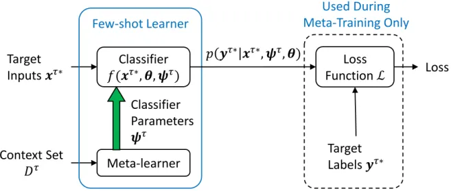
Fig. 2.2 Episodic training. The meta-learner takes the context setDτ as input and induces parameters for the classifierψτ that are specific to taskτ. In addition,θare parameters that are shared across all tasks. Given these parameters, the classifier can now make predictions

p(yτ∗|xτ∗_,ψτ_{,θ) on target inputs x}τ∗_{. If in meta-training mode, the predictions and true} labelsyτ∗ are passed into a loss function and the computed loss can be used to improve the meta-learner parameters via back-propagation.

• Select the number of exampleskcorshotsfor each classc∈Cin the context setDτ.

• Select the number of examplesqcorqueriesfor each classc∈Cin the target setTτ.

• SampleCclasses fromD_trainwithout replacement.

• Form the context setDτby sampling without replacement from each classc∈C,kc

image inputsxτ with labelyτ =c.

• Form the target setTτ by sampling without replacement from each classc∈C,qc

image inputsxτ∗with labelyτ∗=c.

2. Induce a classifier. Feed the context setDτas input to the meta-learner (seeFigure 2.2). The goal of the meta-learner is to process Dτ, and produce a classifier model with parametersθthat are shared across tasks andψτ that are specific to taskτ.

3. Classify. The resulting task-specific classifierf(seeFigure 2.2) can now make predictions

p(yτ∗|xτ∗_,ψτ_{,θ)for any test inputsx}τ∗ _∈Tτ _{associated with the task.}

4. Compute the loss and update the parameters. The predictionsp(yτ∗|xτ∗_,ψτ_{,θ)at the}

true target labelsyτ∗are input to a loss functionLwhere the output loss can be used to back-propagate through the networks and update the parameters of the meta-learner. 5. Iterate. The above steps are repeated until the loss stops decreasing or some other

Meta-testing

1. Same as step 1 in Meta-Training except:

• The task would be drawn from the test setDtest.

• The target setTτ does not require labelsyτ∗. 2. Induce a classifier. Same as step 2 in Meta-Training.

3. Classify. Same as step 3 in Meta-Training.

4. Iterate. Repeat for as many tasks that need to be classified.

Often, the assumption is that meta-test tasks will include classes that have not been seen during meta-training, andDτ will contain only a few observations for each class. In the next section, we cast meta-learning in terms of a probabilistic model.

2.2.3 Hierarchical Probabilistic Modelling View of Meta-Learning

In the previous section, we described the computational flow for a meta-learning approach to multi-task, few-shot classification. In this section, we take a more formal perspective on the scenario.

A general and useful view of meta-learning is through the perspective of hierarchical probabilistic modelling (Heskes,2000;Bakker and Heskes,2003;Grant et al.,2018;Gordon et al.,2019). A standard graphical representation of this modelling approach is presented

inFigure 2.3. Global parametersθ encode information shared across all tasks, while local

parametersψτencode information specific to taskτ. This model introduces ahierarchyof latent parameters, corresponding to the hierarchical nature of the data distribution. LetXτandYτ

denote all the inputs and outputs (both context and target) for taskτ. The joint probability of the outputs and task specific parameters forTtasks, given the inputs and global parameters is:

p {Yτ,ψτ}T_τ=1|{Xτ}T_τ=1,θ = T Y τ=1 p(ψτ|θ) Nτ Y n=1 p(yτ_n|xτ_n,ψτ,θ) Mτ Y m=1 p(y_mτ∗|x_mτ∗,ψτ,θ).

The context setDτ andxτ∗ are always observed andyτ∗ is observed in training. In this thesis, we focus primarily on the posterior predictive distributionp(yτ∗|xτ∗_{, D}τ_{,θ) of the}

model and we make the following assumptions: 1. yτ|xτ _⊥⊥xτ∗

2. p(yτ|xτ_,θ)⊥⊥ψτ

3. yτ∗ ⊥⊥Dτ|ψτ

x

y

ψ

y

x

θ

Context

D

τ

Target

T

τ

m

= 1

, ..., M

n

= 1

, ..., N

τ

=1,...

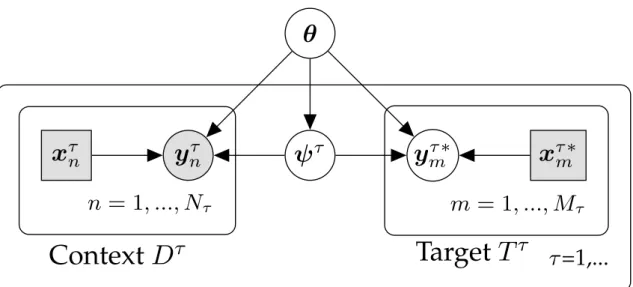
Fig. 2.3 Directed graphical model for multi-task meta-learning that employs shared parameters θ, that are common to all tasks, and task specific parameters{ψτ_}T

τ=1. The data for a taskτ

consists of acontext setDτ ={(x_nτ,yτ_n)}Nτ

n=1 withNτ elements with the inputsxτnand labelsyτn

observed, and atarget setTτ ={(x_mτ∗,y_mτ∗)}Mτ

m=1withMτ elements for which we wish to make

predictions. Here the inputsxτ∗ _{are observed and the labelsy}τ∗ _{are only observed during} training.

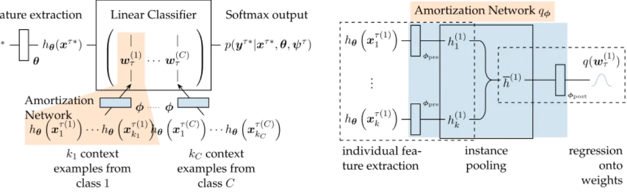
A general approach to meta-learning is to design inference procedures for the task-specific parametersψτ = ψϕ(Dτ)conditioned on the context set (Grant et al.,2018; Gordon et al.,

2019), whereψis parameterized by additional parametersϕ. Thus, a meta-learning algorithm defines a predictive distribution parameterized byθ andϕasp(y_mτ∗|xτ∗

m,ψϕ(Dτ),θ).This

perspective relates to theinnerandouterloops of meta-learning algorithms (Grant et al.,2018; Rajeswaran et al.,2019): the inner loop represents adaptation to a given task by usingψϕto

generate the parametersψτ _{as a function of the context set; while the outer loop represents the}

meta-training objective by computing the loss between predictionsp(yτ∗|xτ∗_,ψ

ϕ(Dτ),θ)for

target inputsxτ∗ and the true target outputsyτ∗ to update the parametersθ andϕthat are shared across tasks.

During meta-training, a taskτ is drawn fromp(τ)and randomly split into a context set

Dτ_{and target setT}τ_{. The meta-learning algorithm’s inner-loop is then applied to the context}

set to produceψτ. Withθandψτ, the algorithm can produce predictions for the target set inputsxτ_m∗. Given a differentiable loss function, and assuming thatψϕis also differentiable,

the meta-learning algorithm can then be trained with stochastic gradient descent algorithms. Using log-likelihood as an example loss function, we may express a meta-learning objective forθandϕas L(θ,ϕ) = _E p(τ) "_Mτ X m=1 logp(y_mτ∗|x_mτ∗,ψϕ(Dτ),θ) # where{{(xτ_m∗,y_mτ∗)}Mτ m=1, D τ_{} ∼p(τ).} (2.1)

In the next section, we use this view to summarize a range of meta-learning approaches.

2.3

Meta-learning Methods

There has been an explosion of few-shot learning algorithms proposed in recent years. For in-depth reviews seeHospedales et al.(2020) andWang et al.(2019). In this section, we will summarize the methods most relevant to this thesis. Typically, few-shot learning approaches are divided into roughly three main approaches including: (i) Gradient-based (ii) Metric Learning (iii) Amortization / Hypernets. However, in this section, we organize various few-shot image classification systems (including our own work) in terms of i) the choice of the parameterization of the classifier (and in particular the nature of the task-specific parameters), and ii) the function used to compute the task-specific parameters from the context set. This space is illustrated inFigure 2.4.

Adaptation Mechanism

Faster at Test-Time

# T

ask

-speci

fic

Par

amet

er

s

Multi-step Gradient Few-step Gradient Semi-Amortized Amortized

Finetune

Residual

Adapters

LEO,

Proto-MAML

CNAP

,

TADAM

VERSA,

Proto Nets,

Matching Nets

MAML

Meta-LSTM

Model Fle

xibility

CAVIA

Disc. k-shot

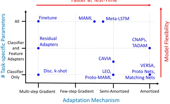
Fig. 2.4 Model design space. They-axis represents the number of task-specific parameters. Increasing the number task-specific parameters increases model flexibility, but also the propen-sity to over-fit. Thex-axis represents the complexity of the mechanism used to adapt the task-specific parameters to training data. On the right areamortizedapproaches (i.e. using fixed functions). On the left is gradient-based adaptation. Mixed approaches lie between. Computational efficiency increases to the right. Flexibility increases to the left, but with it over-fitting and need for hand tuning.

The choice of task-specific parametersψτ. Clearly, any approach to multi-task classification must adapt, at the very least, the top-level classifier layer of the model. A number of successful models have proposed doing just this with e.g., metric-based approaches (Proto Nets (Snell et al.,2017)), variational inference (Disc. k-shot (Bauer et al.,2017)), or amortized networks (VERSA(Gordon et al.,2019) andChapter 3). On the other end of the spectrum are models that adaptallthe parameters of the classifier, e.g., MAML (Finn et al.,2017), Reptile (Nichol et al., 2018), Bayesian MAML (Yoon et al.,2018). The trade-off here is clear: as more parameters are adapted, the resulting model is more flexible, but also slower and more prone to over-fitting. For this reason, in this thesis we will explore methods that modulate only a small portion of the network parameters, following recent work on multi-task learning including Residual Adapters (Rebuffi et al.,2017,2018), and FiLM layers (Perez et al.,2018).

We argue that just adapting the linear classification layer is sufficient when the task distri-bution is not diverse, as in the standard benchmarks used for few-shot classification (Omniglot (Lake et al.,2011) andminiImageNet (Ravi and Larochelle,2017)). However, when faced with a diverse set of tasks, such as that introduced recently byTriantafillou et al.(2020), it is important to adapt the feature extractor on a per-task basis as well.

The adaptation mechanismψ(Dτ). Adaptation varies in the literature from performing full gradient descent learning withDτ (e.g. Fine-tuning (Yosinski et al.,2014)) to relying on simple operations such as taking the mean of class-specific feature representations (Proto Nets, Match-ing Nets (Vinyals et al.,2016)). Recent work has focused on reducing the number of required gradient steps by learning a global initialization (MAML, Reptile) or additional parameters of the optimization procedure (Meta-LSTM (Ravi and Larochelle, 2017)). Gradient-based procedures have the benefit of being flexible, but are computationally demanding, and prone to over-fitting in the low-data regime. Another line of work has focused on learning neural networks to output the values ofψ, which we denote asamortization(VERSA). Amortization greatly reduces the cost of adaptation and enables sharing of global parameters, but may suffer from the amortization gap (Cremer et al.,2018) (i.e., underfitting), particularly in the large data regime. Recent work has proposed using semi-amortized inference (Proto-MAMLTriantafillou et al.(2020), LEO (Rusu et al.,2018)), but have done so while only adapting the classification layer parameters. CNAPS(Requeima et al.,2019b) andChapter 4and TADAM (Oreshkin et al.,2018) use an amortized approach to adapt a key set of feature extractor parameters in addition to the classification layer parameters.

In the following, we group few-shot learning methods in terms of the adaptation mecha-nism, from multi-step gradient through to few-step gradient, and then amortized approaches. We’ll then look at semi-amortized approaches that combine few-step gradient and amortization techniques. We will also cover an additional category that encompasses probabilistic methods that span the categorization above.

2.3.1 Multi-step Gradient Approaches

Multi-step gradient-based approaches for few-shot learning "fine tune" some or all of the parameters in a model to a particular task by taking as many gradient descent training steps using the context set data as necessary to optimize classification accuracy, while trying to avoid over-fitting.

Fine-tuning

A non-episodic baseline to measure meta-learning methods against is referred to asfine-tuning

(Yosinski et al.,2014). Here we pre-train a feature extractor with shared parametersθoff-line on all the classes of the entire meta-learning training setDtrain(i.e. the union of all the training

tasks). The final classifier layer of the pre-trained model is then removed and the remaining layers serve as an embedding function. Note that the meta-training phase is not required when fine-tuning. During meta-testing, for each task, the removed final layer is replaced with an untrained fully-connected layer with input size being equal to the embedding function output dimension and output size equal to the way of the task. The context set data from the test task is then used to train the new final classifier layer (and optionally to update the parameters of the pre-trained embedding function as well) using gradient descent or other optimization method. This network trained on the context set can now be evaluated using the target set data from the task.

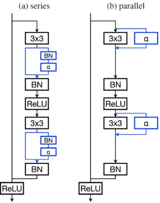
Residual Adapters In addition to fine-tuning the final fully-connected classifier layer,Rebuffi et al.(2017) also fine-tune a small set of key parameters in the feature extractor. In particular, they devise two efficient parameterizations for modulating the output feature maps of 2D convolutional layers in residual neural networks (He et al.,2016) that they callresidual adapters. The idea is to add additional task specific convolution and batch normalization layers with a small number of parameters to a standard residual layer.Figure 2.5depicts both the series and parallel versions of a residual adapter. A compelling aspect is that the new parameterizations result in the majority of the weights of the residual layer being shared across tasks while less than10%of the total weights in a layer are task specific, greatly reducing the number of parameters that need to be fine-tuned compared to adjusting all of the weights in the feature extractor network. The authors demonstrate excellent results on a "visual decathlon" challenge using this approach.

2.3.2 Few-step Gradient Approaches

Few-step gradient-based methods for few-shot learning attempt to learn a good initialization of model parameters such that only a few gradient steps on the context set data are required to fine tune the model to a particular task.

Fig. 2.5 Series (a) versus parallel (b) residual adapters. Standard residual neural network block components are shown in black and the added residual adapter components are shown in blue. Diagram from (Rebuffi et al.,2017)

Model Agnostic Meta-Learning (MAML)

Arguably, the most well-known few-shot learning method is agradient-basedapproach called Model Agnostic Meta-Learning (MAML) (Finn et al.,2017). The basic idea is that a model is initially trained on a variety of tasks such that it can rapidly adapt to any new task by taking only a few additional gradient steps with only a small number of examples from the new task. In a nutshell, their method trains models that can easily be “fine-tuned” to a new task. In other words (referring toFigure 2.2andFigure 2.3), MAML setsθto be the initialization of all the network parameters and the task specific parametersψτare the network parameters after applying one or more gradient steps using the examples in the context setDτ. More specifically, to meta-train MAML, letθbe the (initially random) parameters of the classifierf. Then for each task, compute the task-specific classifier parametersψτby taking one or more

innergradient steps on the context set dataDτwith step sizeα:

Then, update the parametersθby taking ameta(or outer) gradient step with step sizeβon the target set with the classifierf using the task-specific parametersψτ:

θ=θ−β∇_θL(fψτ(xτ∗),yτ∗) (2.3)

NoteEquation (2.3)requires calculating a gradient through a gradient sincef uses the

updated parametersψτ, which can be computationally and memory intensive. There is a

first-order approximation of MAML which performs almost as well with reduced computational complexity.

For meta-testing MAML, equationEquation (2.3)is not necessary and it is replaced with a simple forward pass through the classifier with the task-specific weights:

yτ∗ =fψτ(xτ∗) (2.4)

A key advantage of MAML is that it can work with any model which can be trained with gradient descent. MAML has been applied to classification, regression, and reinforcement learning problems with good success, though recent techniques have surpassed it on stan-dard benchmarks. A downside of MAML is that it requires gradient steps even at meta-test time, which prohibits the use of MAML on mobile devices as common mobile deep learning frameworks currently do not support gradient back-propagation computation. In addition, the original variant of MAML does not provide distributions over parameters or predictions.

InSection 2.3.5we briefly describe some probabilistic variants of MAML, and inChapter 3, we

detail ML-PIP, a distributional model for making predictions that includes MAML as a special case.

Meta-LSTM

(Ravi and Larochelle, 2017) use a Long Short-Term Memory (LSTM) network to learn an optimizer to directly output the task-specific weight updates based on the context set alleviating the need to tune the gradient descent step-size.

Reptile

Nichol et al.(2018) devise an algorithm that is closely related to the first-order variant of MAML, but does not use episodic training (i.e. it does not require the task to be split into context and target sets). Reptile works by computing multiple gradient steps on a task, and moving the network weightsθtowards the fully trained weights on that task so that at test time, only a few gradient steps are required to adapt to the new task.

2.3.3 Amortization via Hypernetworks

A hypernetwork is a network that generates the weights for some or all of another network (Ha et al.,2016). The main challenge in generating the parameters for a high capacity neural network is the large number of weights involved. A fully connected layer with dinputs andkoutputs hasdkweights pluskbiases and a convolutional layer withdinput maps,k

output maps, and filter kernel extentf hasdkf2weights pluskbiases. The key is to devise a parameterization such that the generation network needs to infer only a fraction of the total number of weights in the network.

More typically, in these methods,θparameterizes a shared feature extractor, andψa set of parameters used toadaptthe network to a specific task, which include a linear classifier and possibly additional parameters of the network. These methods are often described asamortized

as the meta-learner learns to learn how to generate classifier parameters incrementally during meta-training across a large number of training tasks. Note that a well known technique called Prototypical Networks (Snell et al.,2017) (described in detail later in this section) can be viewed in this way as: (i) it employs a shared feature extractor to embed inputs in a feature space; and (ii) the computation of the mean embedding vector for each class in the context set can be construed as a simple hypernetwork (with no parameters) that generates the task-specific classifier parameters.

In the following, we summarize the few-shot learning methods that employ amortization. Prior to that we review two technologies that play an important role in the implementation of amortization networks: deep sets and Feature-wise Linear Modulation (FiLM) layers.

Deep-Sets

When processing or learning from a set of elements, it is desirable that the result of the processing or learning is invariant to the ordering of the elements in the set.Zaheer et al.(2017) formalizes the result that a functionf(S)acting on a setSwill be invariant to a permutation in the elements ofS (subject to some restrictions) if it can be decomposed into the form:

f(S) =ρ(X

s∈S

ϕ(s)) (2.5)

whereρandϕare transformations. In practice,ρandϕcan be arbitrary neural networks and the sum inEquation (2.5)can be replaced without loss of generality by a mean operation.Qi et al.(2017) prove (subject to some restrictions) that the sum may also be replaced by amax

operator that takes an arbitrary number of vectors as input and returns a new vector of the element-wise maximum. This concept will prove to be extremely valuable to meta-learning systems as a way tosummarizea dataset. Deep sets are a key component of many amortization networks to achieve invariance to the size and ordering of the context set.

FiLM Layers An effective and economical approach to adapting a convolutional neural network based image classifier to a specific task or dataset is to pretrain the network on a large dataset (such as ImageNet (Krizhevsky et al.,2012)), freeze the learned weights, and then insertadapterlayers with a small number of parameters that will modulate the feature maps at the output of one or more of the convolutional layers in the network. The parameters for the adapter layers can be learned using gradient descent (or some other optimization algorithm) on the context set data or generated by a hypernet using the context set as input. The latter is the approach taken in this research (seeChapter 4).

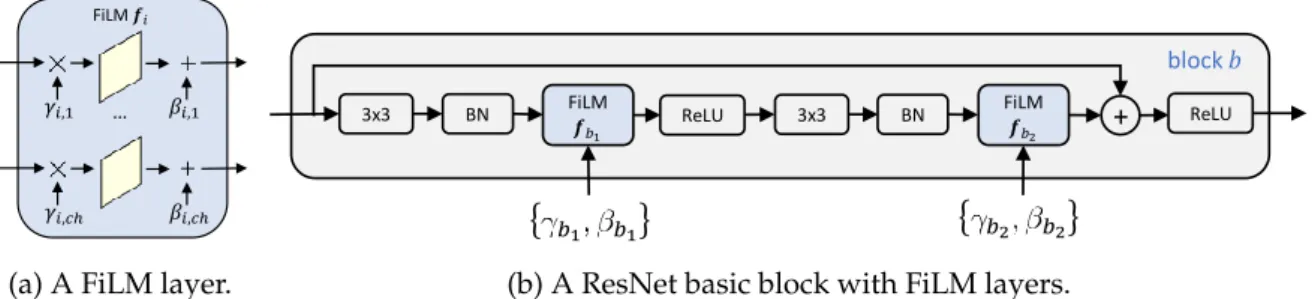
A specific realization of this concept is a Feature-wise Linear Modulation (FiLM) layer (Perez et al., 2018) that scales and shifts the ith feature mapfi of the the output of a 2D

convolutional layer FiLM(fi;γi, βi) =γifi+βi using two parameters,γiandβi.Figure 2.6a

illustrates a FiLM layer operating on a convolutional layer, andFigure 2.6billustrates how a FiLM layer can be added to a standard Residual network block (He et al., 2016). A key advantage of FiLM layers is that they enable expressive feature adaptation while adding even fewer parameters than are required for residual adapters.

FiLM𝒇𝑖

𝛾𝑖,1 𝛽𝑖,1 + 𝛾𝑖,𝑐ℎ 𝛽𝑖,𝑐ℎ

…

(a) A FiLM layer.

3x3 BN FiLM 𝒇𝑏1 ReLU 3x3 BN FiLM 𝒇𝑏2 + ReLU block 𝑏 𝑏1 𝑏1 𝑏2 𝑏2

(b) A ResNet basic block with FiLM layers.

Fig. 2.6 (Left) A FiLM layer operating on convolutional feature maps indexed by channelch. (Right) How a FiLM layer is used within a basic Residual network block (He et al.,2016).

We now summarize specific amortization-based few-shot learning methods. Learnet

Bertinetto et al.(2016) describe a system for generating all the parameters of a feed forward neural network in a single shot. Alearnetnetwork is trained offline and learns to generate the parameters of a secondpupilfeed-forward network that is optimized for 1-shot learning. The key innovation is in the factorization of fully connected and convolutional layers such that there are drastically fewer parameters to predict in the pupil network. The factorization is analogous to singular value decomposition so that a learnet only needs to predict the diagonal elements of the fully connected weight matrix resulting in a reduction fromdkweights to

d. The same concept is extended to convolutional layers resulting in onlydf2weights to be generated instead ofdkf2.

HyperNetworks

Ha et al.(2016) describe a hypernetwork that is able to generate the weights of convolutional, residual, Recurrent Neural Networks (RNNs), and Long Short-Term Memory (LSTM) networks with a dramatic reduction in the number of parameters that need to be generated. To generate a convolutional layer, the hypernetwork learns the weights of two fully-connected linear layers withminputs as well as an embedding vector of sizez such that the number of learnable weights is z+md(z+ 1) +f2k(m+ 1) compared to dkf2. For image classification tasks, the hypernetwork approach leads to only a small increase in error rate when compared to a standard approach.

The following two methods, Prototypical Networks and Matching Networks, are normally categorized asmetric-learningapproaches. Metric learning approaches for few-shot classifi-cation typically map the context set for each task into an embedding space where similar datapoints are clustered together such that a non-parametric classifier that uses a pre-defined distance metric can separate out individual classes and predict their label correctly. However, in our schema, we see these as amortized methods as the generation of the prototypes by computing the mean of the embedding space vectors for each class of the context set can be viewed as an amortization network with no learnable parameters.

Prototypical Networks

Snell et al.(2017) approach few-shot classification by learning a non-linear clustering mapping

gθ to an embedding space and then computing distances to prototype representations of each

class. In particular, the prototype for each classcis simply the mean of the embedding vectors for each class in the context setDτ of taskτ:

Pc= 1 |Dτ c| X xi∈Dτc gθ(xi) (2.6)

Classification of a new target data pointxτ∗ _{is achieved by calculating a softmax over} distances to the learned prototypes:

p(yτ∗ =c|xτ∗,θ) = exp(−d(gθ(x

τ∗_),P

c))

P

c′exp(−d(g_θ(xτ∗),P_c′)) (2.7)

wheredis the euclidean distance function. Figure 2.7is a simple depiction ofEquation (2.7)

for two-way classification. The objective for learning is to minimize the negative log-probability of the actual classcvia gradient descent. Note that other distance functions such as the cosine or Mahalanobis distance could be used in place of the euclidean distance ford.

In the context ofFigure 2.2andFigure 2.3, the parametersθthat are shared across tasks are the parameters of the embedding network g and the parametersψ are the computed prototypesP_candf is a nearest neighbor classifier.

𝒙𝜏∗ 𝑝 𝒚𝜏∗= 1 𝒙𝜏∗, 𝜽) = 𝑒−𝑑1 𝑒−𝑑1+𝑒−𝑑2 𝒫1 𝒫2 𝑑₁ 𝑔𝜽(𝒙𝜏∗) 𝑑₂ 𝑔_𝜽

Fig. 2.7 Two-way classification of an imagexτ∗using Prototypical Networks. The imagexτ∗is first mapped through the feature extractorgθ. Next the distance from the each of the two class

prototypesP1andP2 to the mapped pointgθ(xτ∗)is computed and finally the probability of

the image belonging to class1can be calculated as shown.

As the classification stage in prototypical networks is non-parametric, it is possible to train the model using a certain number of shots per class and way and test the model with different values of shot and way, which adds significant flexibility. The authors found that training with a higher value of way than was used for testing led to superior classification accuracy. In their experiments, they tune the value used for way during training based on validation set results. They hypothesize that training on higher way forces the model to generalize better. However, they also found that there was no advantage to using a different value for shot in training versus testing.

Interestingly, prototypical networks can be shown to be equivalent to a linear classifier with weightsWc,·= 2Pcand biasesbc=−∥Pc∥2(Snell et al.,2017;Triantafillou et al.,2020).

Prototypical Networks can also be viewed as a simple deep sets system - compare the form of the prototype computation inEquation (2.6)to that of deep sets inEquation (2.5).

In summary, prototypical networks are a simple, flexible, efficient approach which achieves state of the art results on certain few-shot learning benchmarks.

Matching Networks

The matching networks model (Vinyals et al.,2016) is conceptually similar to prototypical net-works in that a neural network maps examples into a non-linear embedding space. However, instead of using a euclidean distance based nearest neighbor classifier, matching networks use a weighted nearest neighbor classifier where an LSTM-based attention mechanism determines the weights. When the number of shots is equal to one, prototypical networks and matching networks are equivalent. When the number of shots is greater than one, the two approaches differ due to the attention mechanism in matching networks. The approaches also differ in that prototypical networks use a euclidean distance metric while matching networks use a cosine distance metric. Snell et al.(2017) demonstrate superior accuracy results using a euclidean distance in both approaches.

Few-Shot Image Recognition by Predicting Parameters from Activations

In an approach that has many similarities to Prototypical Networks,Qiao et al.(2018) learn a mappingϕfrom the activations in a pre-trained neural network to the weights of a final layer classifier such that the system is capable of high classification accuracy on both the classes it has been pre-trained on and new classes for which it has seen only a few examples.

More formally (Qiao et al.,2018), letgθ(x)be the activations before the fully connected layer

for a training example imagexon a pre-trained feature extraction network with parametersθ. IfWcare the fully-connected layer weights for classcandPc(refer toEquation (2.6)) are the

mean activations for the classc, thenϕ:→ P_cWc. Note that the 1D weight vectorsWcfor each

classccan be learned independently and subsequently concatenated with each other to form the complete 2D fully connected layer weight matrix.ϕis learned by minimizing the loss:

L(ϕ) = X (c,x)∈D " −ϕ(Pc)gθ(x) + log X c′_∈C eϕ(Pc′)gθ(x) # +λ∥ϕ∥ (2.8)

whereD is a large training set with many examples of each of the classes C and ∥ϕ∥is a regularizer with weightλ. Once trained, this mapping was shown to work well for data from unseen classes in a single forward pass at test time. The activation statistic is not restricted to being the mean - the authors found that the maximum activation was the most effective for unseen classes. Note that this system is also extremely flexible in that a different number of classes can be used at test time due to the context independent construction of the fully-connected classification layer and it is also independent of the number of shots at test time due to that fact that an aggregate statistic of the activations is used as opposed to an activation vector of fixed size.

TADAM: Task dependent adaptive metric for improved few-shot learning

Oreshkin et al.(2018) propose a system using a pre-trained convolutional feature extractor and a prototypical networks based task-specific classifier. The distinguishing feature in the system is a hypernet that takes the context set as input and outputs FiLM layer (Perez et al., 2018) parameters that modulate each of the feature maps that result from the convolutional layers in the feature extractor. The modulation of the activations in the feature extractor allow the pre-trained feature extractor to adapt to the current task, enhancing classification accuracy.

2.3.4 Semi-amortized Approaches

In the context of few-shot learning, semi-amortized methods refer to systems that have some inference parameters that are shared / amortized across many tasks and others that require optimization for each task. In reality, MAML could be construed as semi-amortized as the inner learning rate and the initial network parametersθbefore each inner optimization step

are shared across tasks. That is whyFigure 2.4depicts MAML to be between few-shot gradient and semi-amortized adaptation approaches. Below we summarize few-shot leaning methods that more fully combine amortization networks and few-step gradient optimization to adapt parameters to each task.

Proto-MAML

Proto-MAML (Triantafillou et al.,2020) combines the best of both MAML and Prototypical Networks and demonstrates superior classification accuracy to either of the component meth-ods. Given that the task specific layer of prototypical networks can be expressed as a linear classifier, the Proto-MAML task-specific layer is initialized from the prototypical networks weights and then these weights are updated with gradient steps on the context set using the MAML algorithm.

Met